Bubble Plot

Draw a bubble plot, a scatterplot with varying symbol sizes and colors, or add points to existing plots. A variety of input formats are supported, including vectors, matrices, data frames, formulas, etc.

bubbleplot(x, ...)

# Default S3 method
bubbleplot(x, y, z, std=TRUE, pow=0.5, add=FALSE,
           rev=FALSE, type="p", ylim=NULL, xlab=NULL, ylab=NULL,
           pch=c(16,1), cex.points=1, col="black", bg=par("bg"), ...)

# S3 method for class 'formula'
bubbleplot(formula, data, subset, na.action=NULL, ...)

Arguments

x: a vector of values for the horizontal axis. Can also be a 2-dimensional matrix or table (x values in column names and y values in row names), or a data frame containing x, y, and z in that order. If the data frame contains column names x, y, and z then they will be used for plotting.
...: passed to plot and points.
y: a vector of values for the vertical axis.
z: a vector of values determining the bubble sizes.
std: whether to standardize the z values.
pow: a power coefficient for the bubble sizes.
add: whether to add bubbles to an existing plot.
rev: whether to reverse the y axis.
type: passed to points.
ylim: passed to plot.
xlab, ylab: passed to plot.
pch: passed to points.
cex.points: scales all bubble sizes.
col, bg: passed to points.
formula: has the form z ~ x + y, where z determines the bubble sizes and x and y determine bubble locations.
data: where formula terms are stored, e.g. data frame or list.
subset: a logical vector specifying which data to plot.
na.action: how NA values are handled.

Details

The std standardization sets z = abs(z) / mean(abs(z)).

The pow = 0.5 (square root) is a good default, where a z value of 2 has twice the area of 1. See example #2 below for an exception, where the z value is tree circumference and therefore proportional to the tree diameter.

The pch, col, and bg arguments can be be vectors of length 2, where positive z values are drawn with pch[1], col[1], bg[1] and negative z values are drawn with pch[2], col[2], and bg[2].

Author

Arni Magnusson.

Examples

catch.t <- xtabs(Catch~Year+Age, catch.d)              # example table
catch.m <- as.matrix(as.data.frame(unclass(catch.t)))  # example matrix

# 1  Formula
bubbleplot(Catch~Age+Year, data=catch.d)

# Use rev=TRUE to get same layout as crosstab matrix:
print(catch.m)
#>         3     4    5     6     7    8    9   10  11  12  13  14
#> 1980  275  2540 5214  2596  2169 1341  387  262 155 112  64  33
#> 1981  203  1325 3503  5404  1457 1415  578  242  61 154 135 128
#> 1982  508  1092 2804  4845  4293 1215  975  306  59  35  48  46
#> 1983  107  1750 1065  2455  4454 2311  501  251  38  12   2   4
#> 1984   53   657  800  1825  2184 3610  844  376 291 135 185 226
#> 1985  376  4014 3366  1958  1536 1172  747  479  74  23  72  71
#> 1986 3108  1400 4170  2665  1550 1116  628 1549 216  51  30  14
#> 1987  956  5135 4428  5409  2915 1348  661  496 498  58  27  48
#> 1988 1318  5067 6619  3678  2859 1775  845  226 270 107  24   1
#> 1989  315  4313 8471  7309  1794 1928  848  270 191 135  76  10
#> 1990  143  1692 5471 10112  6174 1816 1087  380 151  55  76  37
#> 1991  198   874 3613  6844 10772 3223  858  838 228  40   6   5
#> 1992  242  2928 3844  4355  3884 4046 1290  350 196  56  54  15
#> 1993  657  1083 2841  2252  2247 2314 3671  830 223 188  81  12
#> 1994  702  2955 1770  2603  1377 1243 1263 2009 454 158 188  82
#> 1995 1573  1853 2661  1807  2370  905  574  482 521 106  35  13
#> 1996 1102  2608 1868  1649   835 1233  385  267 210 232 141  74
#> 1997  603  2960 2766  1651  1178  599  454  125  95 114  77  43
#> 1998  183  1289 1767  1545  1114  658  351  265 120  81  85  85
#> 1999  989   732 1564  2176  1934  669  324  140  72  25  28  22
#> 2000  850  2383  896  1511  1612 1806  335  173  57  33  17   7
#> 2001 1223  2619 2184   591   977  943  819  186  94  28  28  13
#> 2002 1187  4190 3147  2970   519  820  570  309 101  27  15  11
#> 2003 2284  4363 6031  2472  1942  285  438  289 196  28  29  15
#> 2004  952  7841 7195  5363  1563 1057  211  224 157  74  39  11
#> 2005 2607  3089 7333  6876  3592  978  642  119 149  89  46  12
#> 2006 1380 10051 2616  5840  4514 1989  667  485 118 112  86  31
#> 2007 1244  6552 8751  2124  2935 1817  964  395 190  43  36  20
#> 2008 1432  3602 5874  6706  1155 1894 1248  803 262 176  87  44
#> 2009 2820  5166 2084  2734  2883  777 1101  847 555 203 134  36
#> 2010 2146  6284 3058   997  1644 1571  514  656 522 231 114  64
#> 2011 2004  4850 4006  1502   677 1065 1145  323 433 244 150  75
#> 2012 1183  4816 3514  2417   903  432  883 1015 354 277 173  99
#> 2013 1163  5538 6366  2963  1610  664  375  537 460 124 118  78
#> 2014  668  3499 4867  2805  1276  725  347  241 312 199 128  74
bubbleplot(Catch~Age+Year, data=catch.d, rev=TRUE, las=1)


# 2  Data frame
bubbleplot(catch.d)

bubbleplot(Orange)

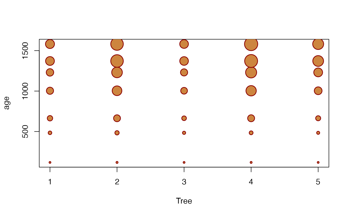
# Visualize tree transverse section at breast height
bubbleplot(Orange, pow=1, cex=2, pch=21,
           col="darkred", bg="peru", lwd=1.5)


# 3  Matrix or table
bubbleplot(catch.m)

bubbleplot(catch.t)


# 4  Positive and negative values
bubbleplot(catch.r)

bubbleplot(Resid~Age+Year, catch.r, subset=Age %in% 4:9,
           rev=TRUE, xlim=c(3.5,9.5), cex=1.3)
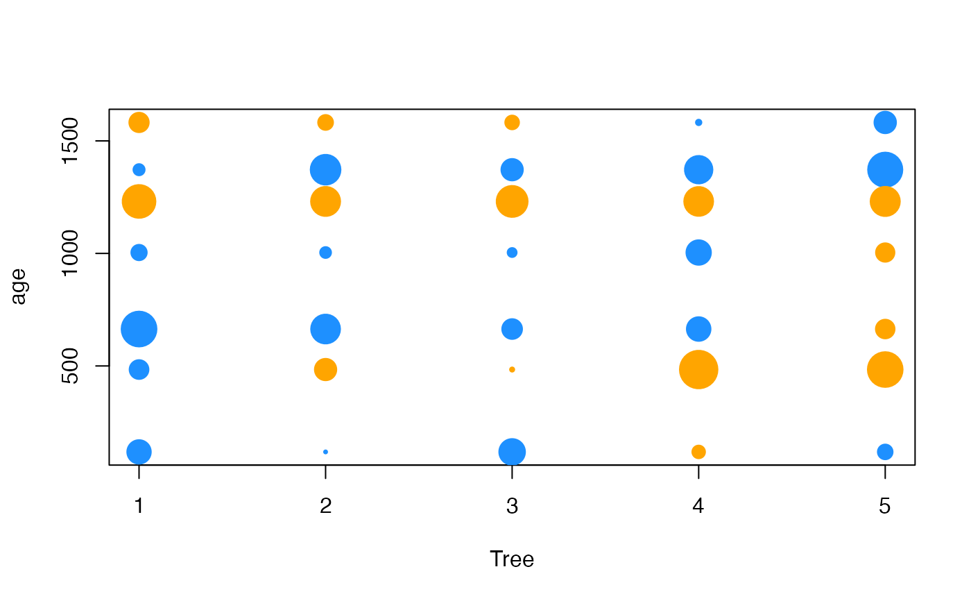
# Residuals from orange tree model
library(nlme)

fm <- nlme(circumference~phi1/(1+exp(-(age-phi2)/phi3)),
           fixed=phi1+phi2+phi3~1, random=phi1~1|Tree,
           data=Orange, start=c(phi1=200,phi2=800,phi3=400))
bubbleplot(residuals(fm)~Tree+age, Orange)

bubbleplot(residuals(fm)~Tree+age, Orange, cex=2.5, pch=16,
           col=c("dodgerblue","orange"))


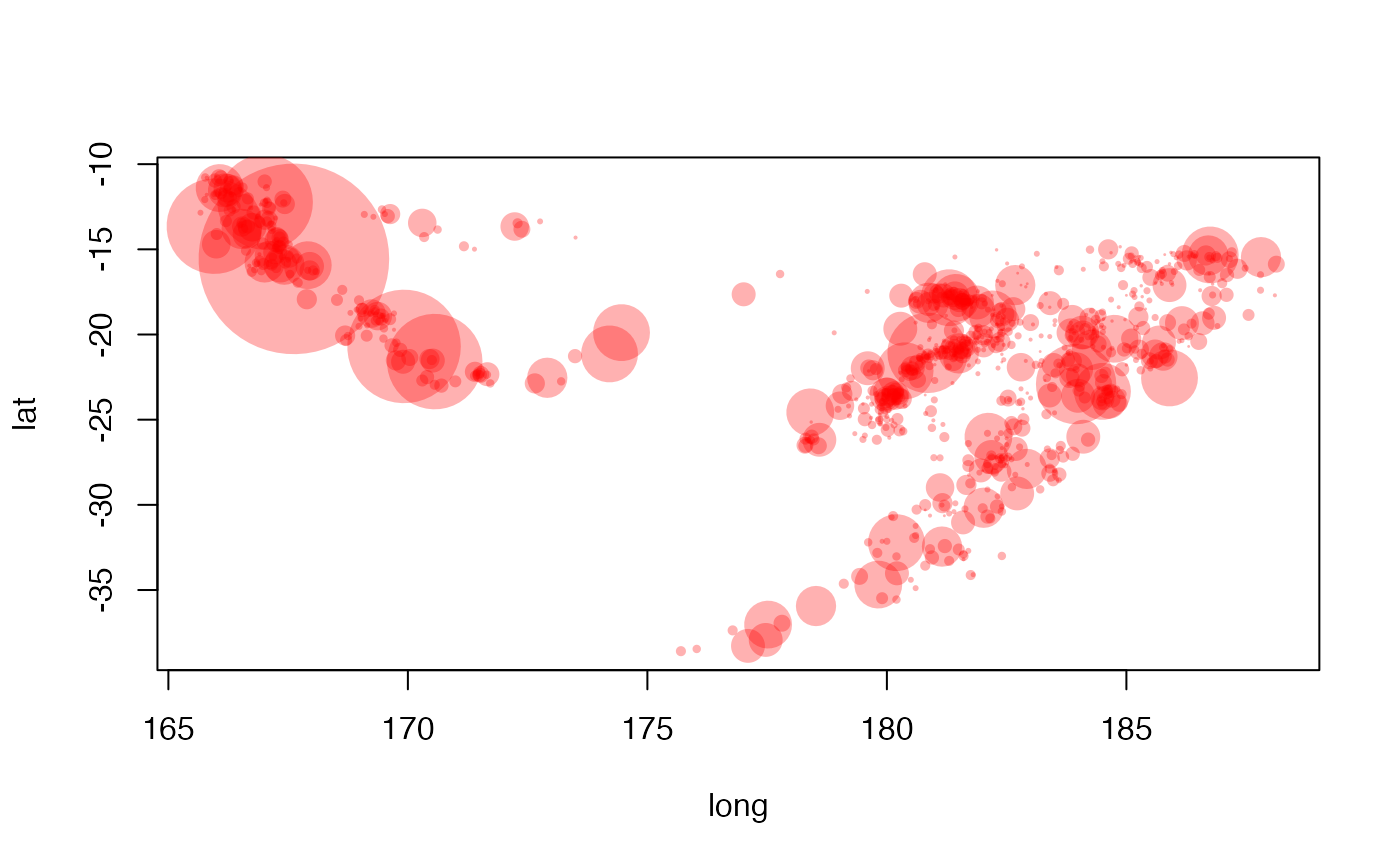
# 5  Richter magnitude, amplitude, and energy release
bubbleplot(mag~long+lat, quakes, pch=1)

bubbleplot(10^mag~long+lat, quakes, cex=1.2, col=gray(0, 0.3))

bubbleplot(sqrt(1000)^mag~long+lat, quakes, cex=1.2, col=gray(0, 0.3))

bubbleplot(sqrt(1000)^mag~long+lat, quakes, cex=1.2, col="#FF00004D")

Arguments

Details

Author

See also

Examples