Compute and Plot a 2-Dimensional Histogram
hist2d.RdCompute and plot a 2-dimensional histogram.
hist2d(x,y=NULL, nbins=200, same.scale=FALSE, na.rm=TRUE, show=TRUE,
       col=c("black", heat.colors(12)), FUN=base::length, xlab, ylab,
       ... )
# S3 method for class 'hist2d'
print(x, ...)
Arguments
- x
either a vector containing the x coordinates or a matrix with 2 columns.
- y
a vector contianing the y coordinates, not required if `x' is matrix
- nbins
number of bins in each dimension. May be a scalar or a 2 element vector. Defaults to 200.
- same.scale
use the same range for x and y. Defaults to FALSE.
- na.rm
Indicates whether missing values should be removed. Defaults to TRUE.
- show
Indicates whether the histogram be displayed using
imageonce it has been computed. Defaults to TRUE.- col
Colors for the histogram. Defaults to "black" for bins containing no elements, a set of 16 heat colors for other bins.
- FUN
Function used to summarize bin contents. Defaults to
base::length. Use, e.g.,meanto calculate means for each bin instead of counts.- xlab,ylab
(Optional) x and y axis labels
- ...
Parameters passed to the image function.
Details
This fucntion creates a 2-dimensional histogram by cutting the x and
y dimensions into nbins sections. A 2-dimensional matrix is
then constucted which holds the counts of the number of observed (x,y) pairs
that fall into each bin. If show=TRUE, this matrix is then
then passed to image for display.
Value
A list containing 5 elements:
- counts
Matrix containing the number of points falling into each bin
- x.breaks, y.breaks
Lower and upper limits of each bin
- x,y
midpoints of each bin
Examples
## example data, bivariate normal, no correlation
x <- rnorm(2000, sd=4)
y <- rnorm(2000, sd=1)
## separate scales for each axis, this looks circular
hist2d(x,y)
 #>
#> ----------------------------
#> 2-D Histogram Object
#> ----------------------------
#>
#> Call: hist2d(x = x, y = y)
#>
#> Number of data points: 2000
#> Number of grid bins: 200 x 200
#> X range: ( -12.89785 , 14.65185 )
#> Y range: ( -3.439596 , 3.536622 )
#>
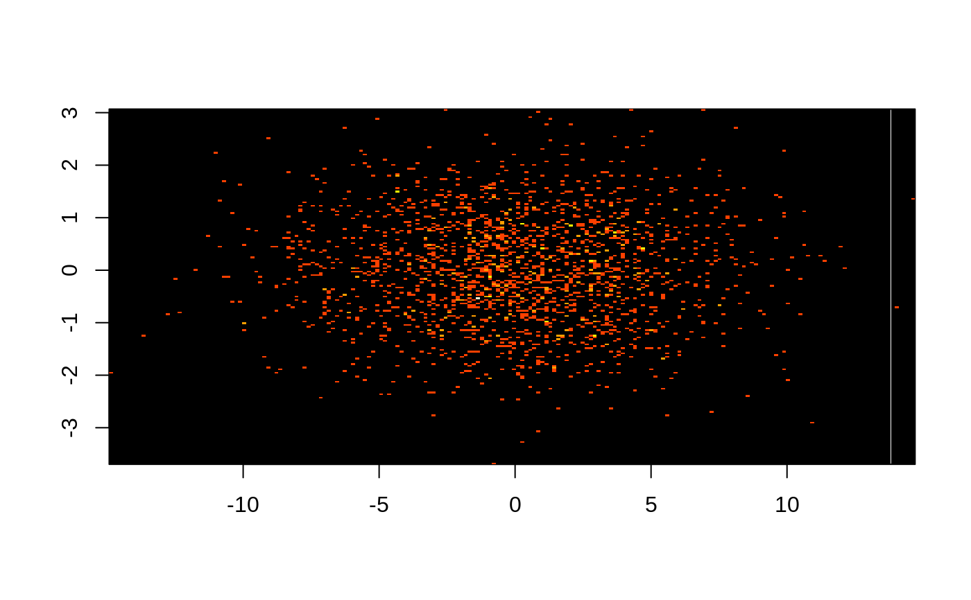
## same scale for each axis, this looks oval
hist2d(x,y, same.scale=TRUE)
#>
#> ----------------------------
#> 2-D Histogram Object
#> ----------------------------
#>
#> Call: hist2d(x = x, y = y)
#>
#> Number of data points: 2000
#> Number of grid bins: 200 x 200
#> X range: ( -12.89785 , 14.65185 )
#> Y range: ( -3.439596 , 3.536622 )
#>
## same scale for each axis, this looks oval
hist2d(x,y, same.scale=TRUE)
 #>
#> ----------------------------
#> 2-D Histogram Object
#> ----------------------------
#>
#> Call: hist2d(x = x, y = y, same.scale = TRUE)
#>
#> Number of data points: 2000
#> Number of grid bins: 200 x 200
#> X range: ( -12.89785 , 14.65185 )
#> Y range: ( -12.89785 , 14.65185 )
#>
## use different ## bins in each dimension
hist2d(x,y, same.scale=TRUE, nbins=c(100,200) )
#>
#> ----------------------------
#> 2-D Histogram Object
#> ----------------------------
#>
#> Call: hist2d(x = x, y = y, same.scale = TRUE)
#>
#> Number of data points: 2000
#> Number of grid bins: 200 x 200
#> X range: ( -12.89785 , 14.65185 )
#> Y range: ( -12.89785 , 14.65185 )
#>
## use different ## bins in each dimension
hist2d(x,y, same.scale=TRUE, nbins=c(100,200) )
 #>
#> ----------------------------
#> 2-D Histogram Object
#> ----------------------------
#>
#> Call: hist2d(x = x, y = y, nbins = c(100, 200), same.scale = TRUE)
#>
#> Number of data points: 2000
#> Number of grid bins: 100 x 200
#> X range: ( -12.89785 , 14.65185 )
#> Y range: ( -12.89785 , 14.65185 )
#>
## use the hist2d function to create an h2d object
h2d <- hist2d(x,y,show=FALSE, same.scale=TRUE, nbins=c(20,30))
## show object summary
h2d
#>
#> ----------------------------
#> 2-D Histogram Object
#> ----------------------------
#>
#> Call: hist2d(x = x, y = y, nbins = c(20, 30), same.scale = TRUE, show = FALSE)
#>
#> Number of data points: 2000
#> Number of grid bins: 20 x 30
#> X range: ( -12.89785 , 14.65185 )
#> Y range: ( -12.89785 , 14.65185 )
#>
## object contents
str(h2d)
#> List of 7
#> $ counts : num [1:20, 1:30] 0 0 0 0 0 0 0 0 0 0 ...
#> ..- attr(*, "dimnames")=List of 2
#> .. ..$ : chr [1:20] "[-12.9,-11.5]" "(-11.5,-10.1]" "(-10.1,-8.77]" "(-8.77,-7.39]" ...
#> .. ..$ : chr [1:30] "[-12.9,-12]" "(-12,-11.1]" "(-11.1,-10.1]" "(-10.1,-9.22]" ...
#> $ x.breaks: num [1:21] -12.9 -11.52 -10.14 -8.77 -7.39 ...
#> $ y.breaks: num [1:31] -12.9 -11.98 -11.06 -10.14 -9.22 ...
#> $ x : num [1:20] -12.21 -10.83 -9.45 -8.08 -6.7 ...
#> $ y : num [1:30] -12.44 -11.52 -10.6 -9.68 -8.77 ...
#> $ nobs : int 2000
#> $ call : language hist2d(x = x, y = y, nbins = c(20, 30), same.scale = TRUE, show = FALSE)
#> - attr(*, "class")= chr "hist2d"
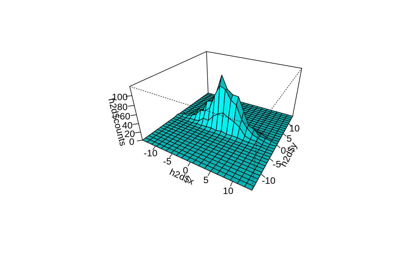
## perspective plot
persp( h2d$x, h2d$y, h2d$counts,
ticktype="detailed", theta=30, phi=30,
expand=0.5, shade=0.5, col="cyan", ltheta=-30)
#>
#> ----------------------------
#> 2-D Histogram Object
#> ----------------------------
#>
#> Call: hist2d(x = x, y = y, nbins = c(100, 200), same.scale = TRUE)
#>
#> Number of data points: 2000
#> Number of grid bins: 100 x 200
#> X range: ( -12.89785 , 14.65185 )
#> Y range: ( -12.89785 , 14.65185 )
#>
## use the hist2d function to create an h2d object
h2d <- hist2d(x,y,show=FALSE, same.scale=TRUE, nbins=c(20,30))
## show object summary
h2d
#>
#> ----------------------------
#> 2-D Histogram Object
#> ----------------------------
#>
#> Call: hist2d(x = x, y = y, nbins = c(20, 30), same.scale = TRUE, show = FALSE)
#>
#> Number of data points: 2000
#> Number of grid bins: 20 x 30
#> X range: ( -12.89785 , 14.65185 )
#> Y range: ( -12.89785 , 14.65185 )
#>
## object contents
str(h2d)
#> List of 7
#> $ counts : num [1:20, 1:30] 0 0 0 0 0 0 0 0 0 0 ...
#> ..- attr(*, "dimnames")=List of 2
#> .. ..$ : chr [1:20] "[-12.9,-11.5]" "(-11.5,-10.1]" "(-10.1,-8.77]" "(-8.77,-7.39]" ...
#> .. ..$ : chr [1:30] "[-12.9,-12]" "(-12,-11.1]" "(-11.1,-10.1]" "(-10.1,-9.22]" ...
#> $ x.breaks: num [1:21] -12.9 -11.52 -10.14 -8.77 -7.39 ...
#> $ y.breaks: num [1:31] -12.9 -11.98 -11.06 -10.14 -9.22 ...
#> $ x : num [1:20] -12.21 -10.83 -9.45 -8.08 -6.7 ...
#> $ y : num [1:30] -12.44 -11.52 -10.6 -9.68 -8.77 ...
#> $ nobs : int 2000
#> $ call : language hist2d(x = x, y = y, nbins = c(20, 30), same.scale = TRUE, show = FALSE)
#> - attr(*, "class")= chr "hist2d"
## perspective plot
persp( h2d$x, h2d$y, h2d$counts,
ticktype="detailed", theta=30, phi=30,
expand=0.5, shade=0.5, col="cyan", ltheta=-30)
 ## for contour (line) plot ...
contour( h2d$x, h2d$y, h2d$counts, nlevels=4 )
## for contour (line) plot ...
contour( h2d$x, h2d$y, h2d$counts, nlevels=4 )
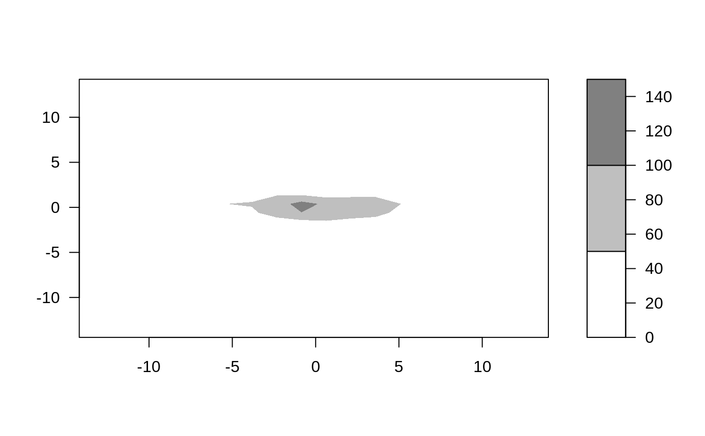
 ## for a filled contour plot ...
filled.contour( h2d$x, h2d$y, h2d$counts, nlevels=4,
col=gray((4:0)/4) )
## for a filled contour plot ...
filled.contour( h2d$x, h2d$y, h2d$counts, nlevels=4,
col=gray((4:0)/4) )