Plot multiple variables on the same region, with appropriate axes

overplot graphs a set of variables defined on the same x-range but which have varying y-ranges on the same plotting area. For each set of y-values it uses a different color and line-type and and draws a correspondingly colored and line-typed axis. panel.overplot is used by overplot to draw the individual graphs.

overplot(formula, data = parent.frame(), same.scale = FALSE, xlab, ylab,
         xlim, ylim, min.y, max.y, log = "", panel = "panel.overplot",
         subset, plot = TRUE, groups, main, f = 2/3, ...)

Arguments

formula: Formula describing the x and y variables. It should be of the form x ~ y|z. The conditioning variable (z) should be a factor.
same.scale: Logical value indicating whether the plot region should have the same range for all plots. Defaults to FALSE.
xlab, ylab, xlim, ylim, main: Standard plotting parameters. See plot for details
min.y, max.y: Scalar or vector values used to specify the y plotting limits for individual plots. If a single scalar value is provided, it will be used for all plots. These parameters can be used specify one end of the individual plot ranges, while allowing the other end to vary with the data. EG, to force 0 to always be within the plot region.
log: character string ”, 'x', 'y', or 'xy', indicating which axes should be plotted on a log scale. Defaults to ” (neither).
panel: a plotting function to be called to draw the individual plots. Defaults to overplot.panel, which plots the points and a lowess smooth.
plot: Logical value indicating whether to draw the plot.
groups: (optional) character vector giving the names of levels of the conditioning variable to plot. Defaults to all levels of the conditioning variable.
f: Smoothing parameter for lowess
data, subset, ...: parameters passed to model.frame to obtain the data to be plotted from the formula.

Details

This function essentially performs

tmp <- split(data, z)

for(i in levels(z))

plot( x ~ y, data=tmp[[z]] )

except that all of the plots are shown on the same plotting region and varying scales for each value of z are handled nicely.

Value

A copy of the data split by the conditioning variable.

Author

Gregory R. Warnes greg@warnes.net

Examples


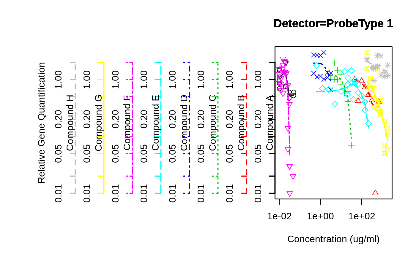
# Example teratogenicity rtPCR data
data(rtPCR)

# same scale
overplot( RQ ~ Conc..ug.ml. | Test.Substance,
         data=rtPCR,
         subset=Detector=="ProbeType 1" & Conc..ug.ml. > 0,
         same.scale=TRUE,
         log="xy",
         f=3/4,
         main="Detector=ProbeType 1",
         xlab="Concentration (ug/ml)",
         ylab="Relative Gene Quantification"
         )


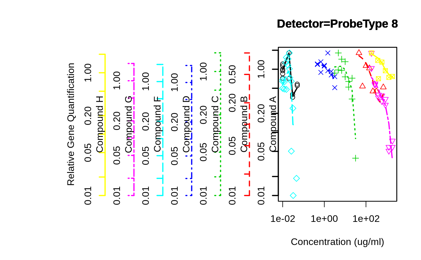
# different scales, but force lower limit to 0.01 
overplot( RQ ~ Conc..ug.ml. | Test.Substance,
         data=rtPCR,
         subset=Detector=="ProbeType 8" & Conc..ug.ml. > 0,
         log="xy",
         f=3/4,
         main="Detector=ProbeType 8",
         xlab="Concentration (ug/ml)",
         ylab="Relative Gene Quantification",
         min.y=0.01
         )
#> Warning: 1 y value <= 0 omitted from logarithmic plot
#> Warning: 1 y value <= 0 omitted from logarithmic plot