Enhanced Heat Maps with heatmap.2
Andy Liaw, original; R. Gentleman, M. Maechler, W. Huber, G. Warnes, revisions. Tal Galili
2025-11-29
Source:vignettes/heatmap.2.Rmd
heatmap.2.RmdIntroduction
The heatmap.2 function provides an enhanced version of
the standard R heatmap function with numerous additional
features and customization options. This vignette demonstrates the key
capabilities and usage patterns of heatmap.2. It is based
on the manual for ?heatmap.2, written by Andy Liaw,
original; R. Gentleman, M. Maechler, W. Huber, G. Warnes, revisions.
Details on Dendrograms, Scaling, and Plot Layout
Dendrogram Behavior (Rowv, Colv)
- If either
RowvorColvare already dendrograms, they are honored and their ordering is preserved (not reordered). - Otherwise, dendrograms are computed as , where is either or .
- If either is a vector (of “weights”), the appropriate dendrogram () is reordered according to the supplied values, subject to the constraints imposed by the dendrogram, using (in the row case).
- If either is missing (as by default), the ordering of the corresponding dendrogram is by the mean value of the rows/columns (e.g., in the row case).
- If either is
NULL, no reordering will be done for the corresponding side.
Data Scaling (scale)
- If
scale="row"(orscale="col"), the rows (columns) are scaled to have mean zero and standard deviation one. - This scaling has some empirical evidence of being useful in genomic plotting.
Color Selection
- The default colors range from red to white () and are generally not considered aesthetically pleasing.
- Consider using enhancements like the RColorBrewer package to select better colors.
Plot Layout (Default and Customization)
- By default, four components are displayed in the
plot:
- Top left: The color key.
- Top right: The column dendrogram.
- Bottom left: The row dendrogram.
- Bottom right: The image plot (heatmap).
- When
RowSideColororColSideColorare provided, an additional row or column is inserted in the appropriate location. - This layout can be overridden by specifying appropriate values for
lmat,lwid, andlhei:-
lmatcontrols the relative position of each element. -
lwidcontrols the column width. -
lheicontrols the row height.
-
- See the help page for
layoutfor details on how to use these arguments.
Note
- The original rows and columns are reordered to
match the dendrograms
RowvandColv(if present). -
heatmap.2()useslayoutto arrange the plot elements. Consequentially, it cannot be used in a multi-column/row layout usinglayout(...),par(mfrow=...)or(mfcol=...).
Load Data
Dendrogram Options
demonstrate the effect of row and column dendrogram options
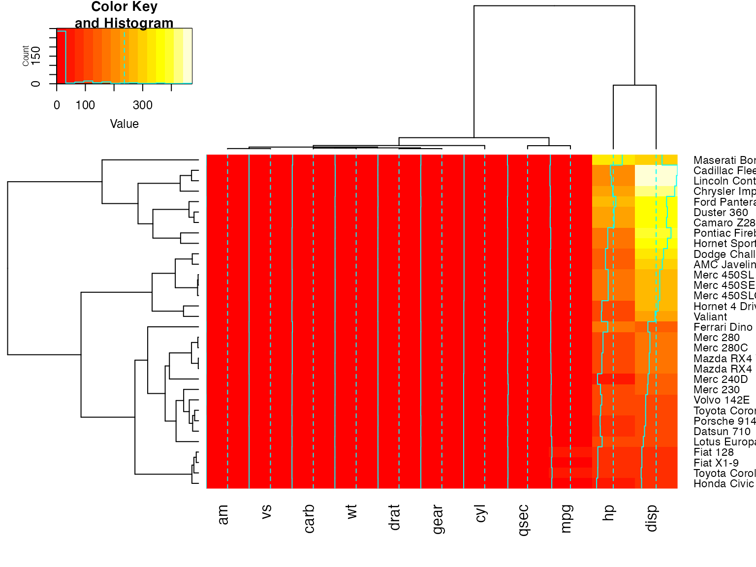
heatmap.2(x) ## default - dendrogram plotted and reordering done.
heatmap.2(x, dendrogram="none") ## no dendrogram plotted, but reordering done.
heatmap.2(x, dendrogram="row") ## row dendrogram plotted and row reordering done.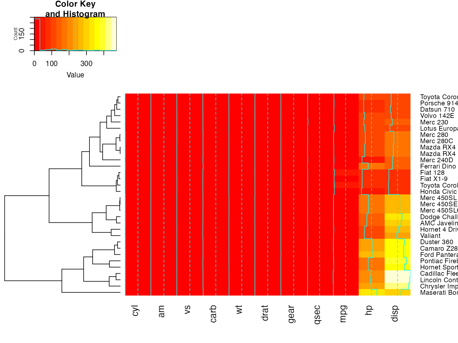
heatmap.2(x, dendrogram="col") ## col dendrogram plotted and col reordering done.
heatmap.2(x, keysize=2) ## default - dendrogram plotted and reordering done.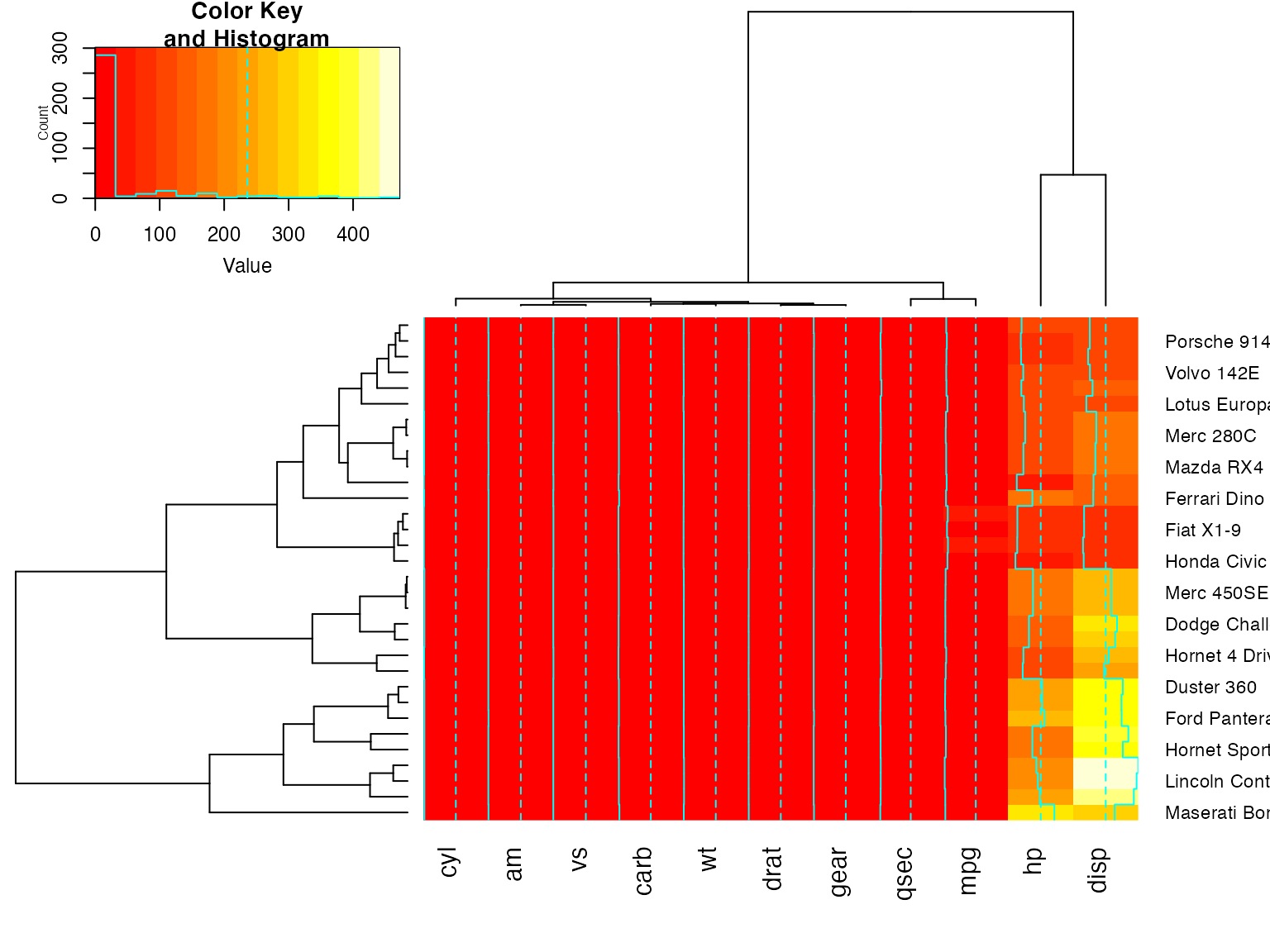
heatmap.2(x, Rowv=FALSE, dendrogram="both") ## generates a warning!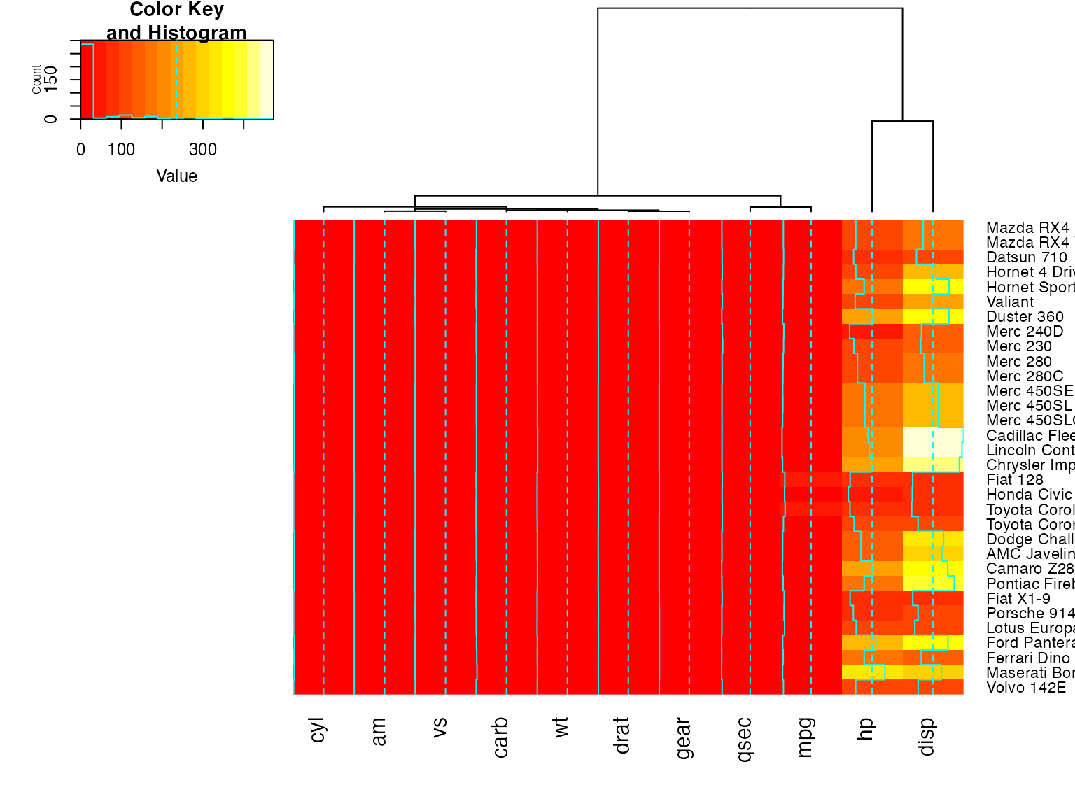
heatmap.2(x, Rowv=NULL, dendrogram="both")  ## generates a warning!
heatmap.2(x, Colv=FALSE, dendrogram="both") ## generates a warning!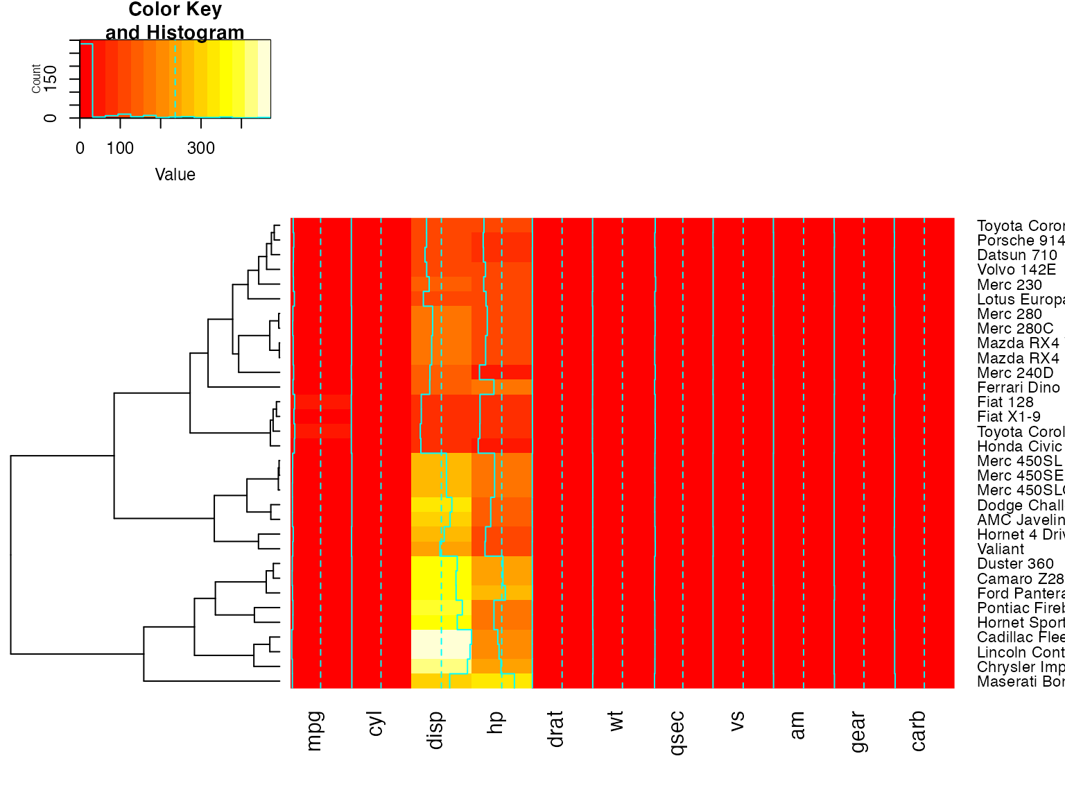
Color dendrograms’ branches (using dendextend)
full <- heatmap.2(x) # we use it to easily get the dendrograms
library(dendextend)  # for color_branches
heatmap.2(x,
        Rowv=color_branches(full$rowDendrogram, k = 3),
        Colv=color_branches(full$colDendrogram, k = 2))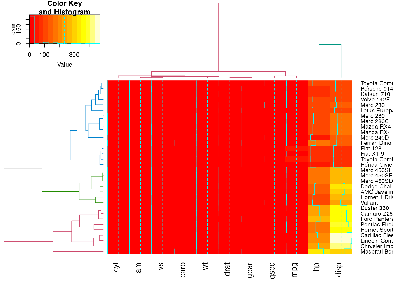
# Look at the vignette for more details:
# https://cran.r-project.org/web/packages/dendextend/vignettes/dendextend.html
plot a sub-cluster using the same color coding as for the full heatmap
full <- heatmap.2(x)
heatmap.2(x, Colv=full$colDendrogram[[2]], breaks=full$breaks) # column subset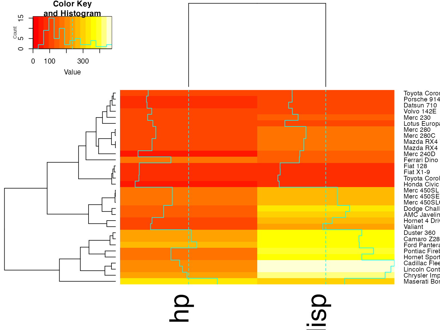
heatmap.2(x, Rowv=full$rowDendrogram[[1]], breaks=full$breaks) # row subset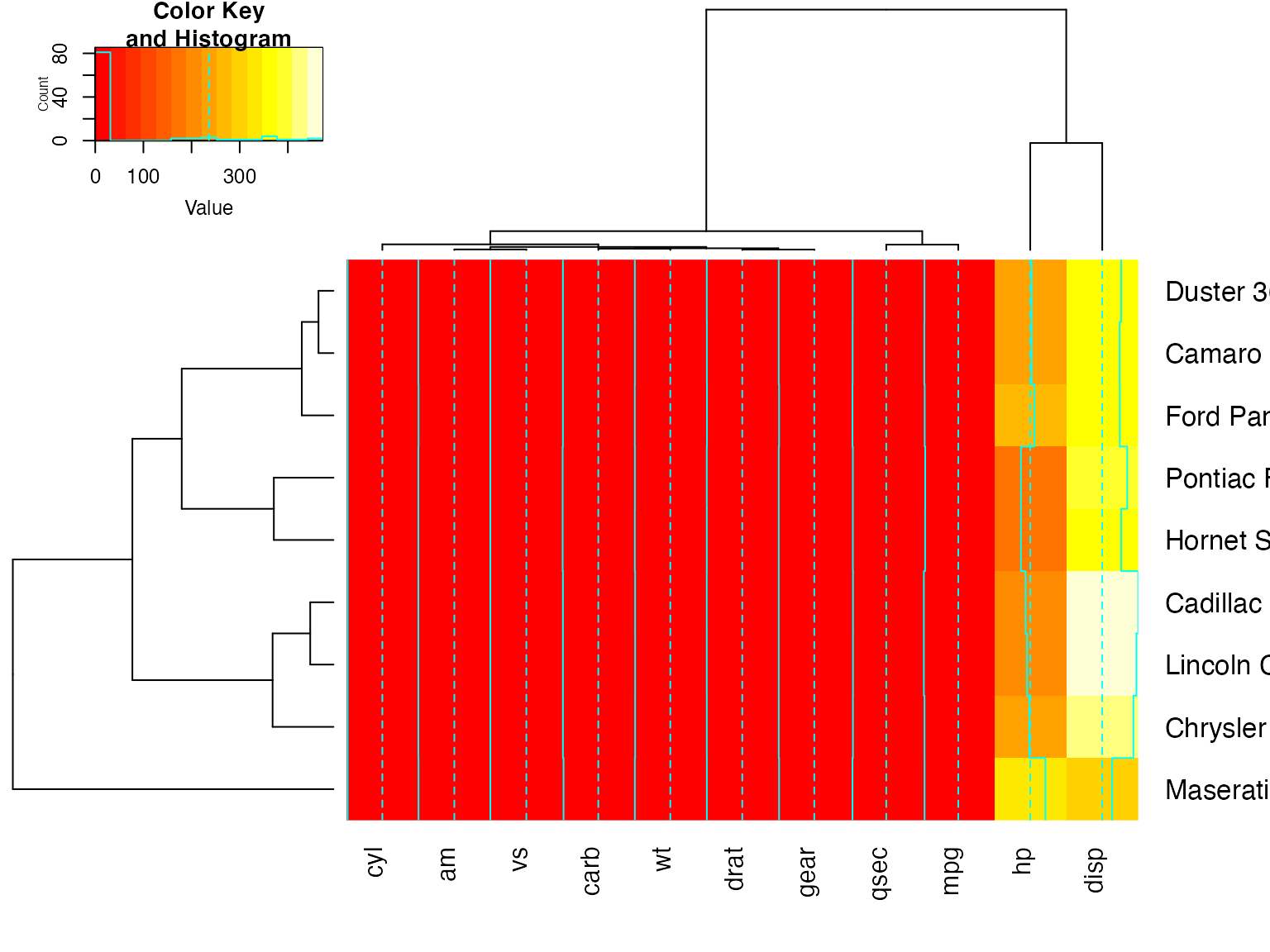
heatmap.2(x, Colv=full$colDendrogram[[2]],
            Rowv=full$rowDendrogram[[1]], breaks=full$breaks)  # both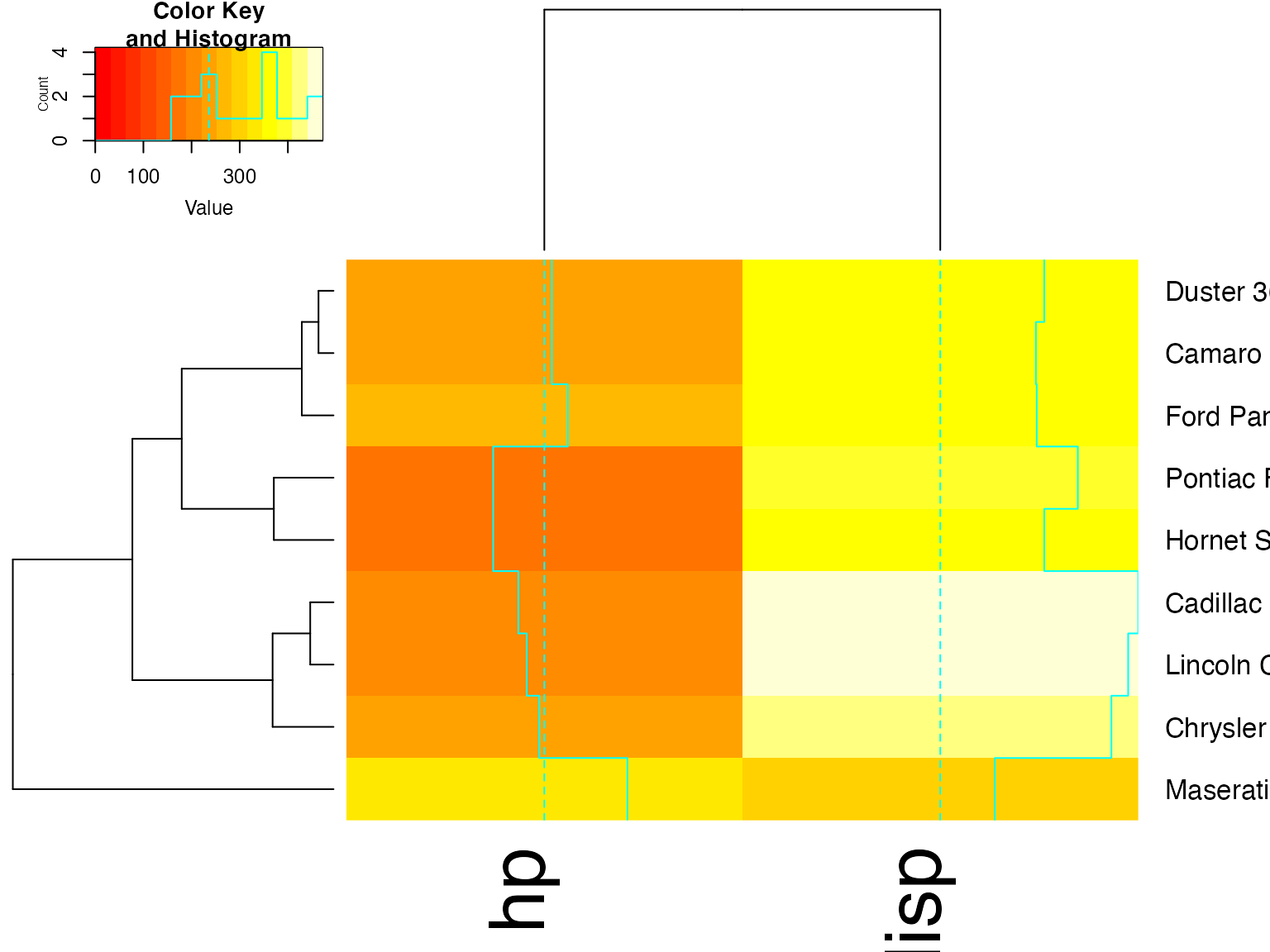


Show effect of offsetRow/offsetCol (only works when srtRow/srtCol is
## not also present)
heatmap.2(x, offsetRow=0, offsetCol=0)
heatmap.2(x, offsetRow=1, offsetCol=1)
heatmap.2(x, offsetRow=2, offsetCol=2)
heatmap.2(x, offsetRow=-1, offsetCol=-1)
heatmap.2(x, srtRow=0, srtCol=90, offsetRow=0, offsetCol=0)
heatmap.2(x, srtRow=0, srtCol=90, offsetRow=1, offsetCol=1)
heatmap.2(x, srtRow=0, srtCol=90, offsetRow=2, offsetCol=2)
heatmap.2(x, srtRow=0, srtCol=90, offsetRow=-1, offsetCol=-1)
Show how to use ‘extrafun’ to replace the ‘key’ with a scatterplot
lmat <- rbind( c(5,3,4), c(2,1,4) )
lhei <- c(1.5, 4)
lwid <- c(1.5, 4, 0.75)

myplot <- function() {
           oldpar <- par("mar")
           par(mar=c(5.1, 4.1, 0.5, 0.5))
           plot(mpg ~ hp, data=x)
         }

heatmap.2(x, lmat=lmat, lhei=lhei, lwid=lwid, key=FALSE, extrafun=myplot)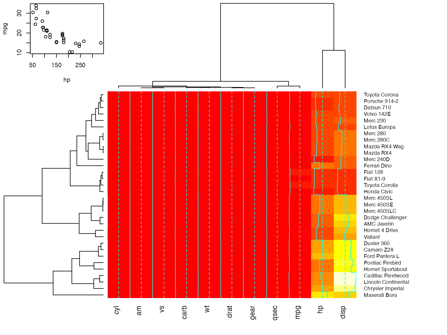
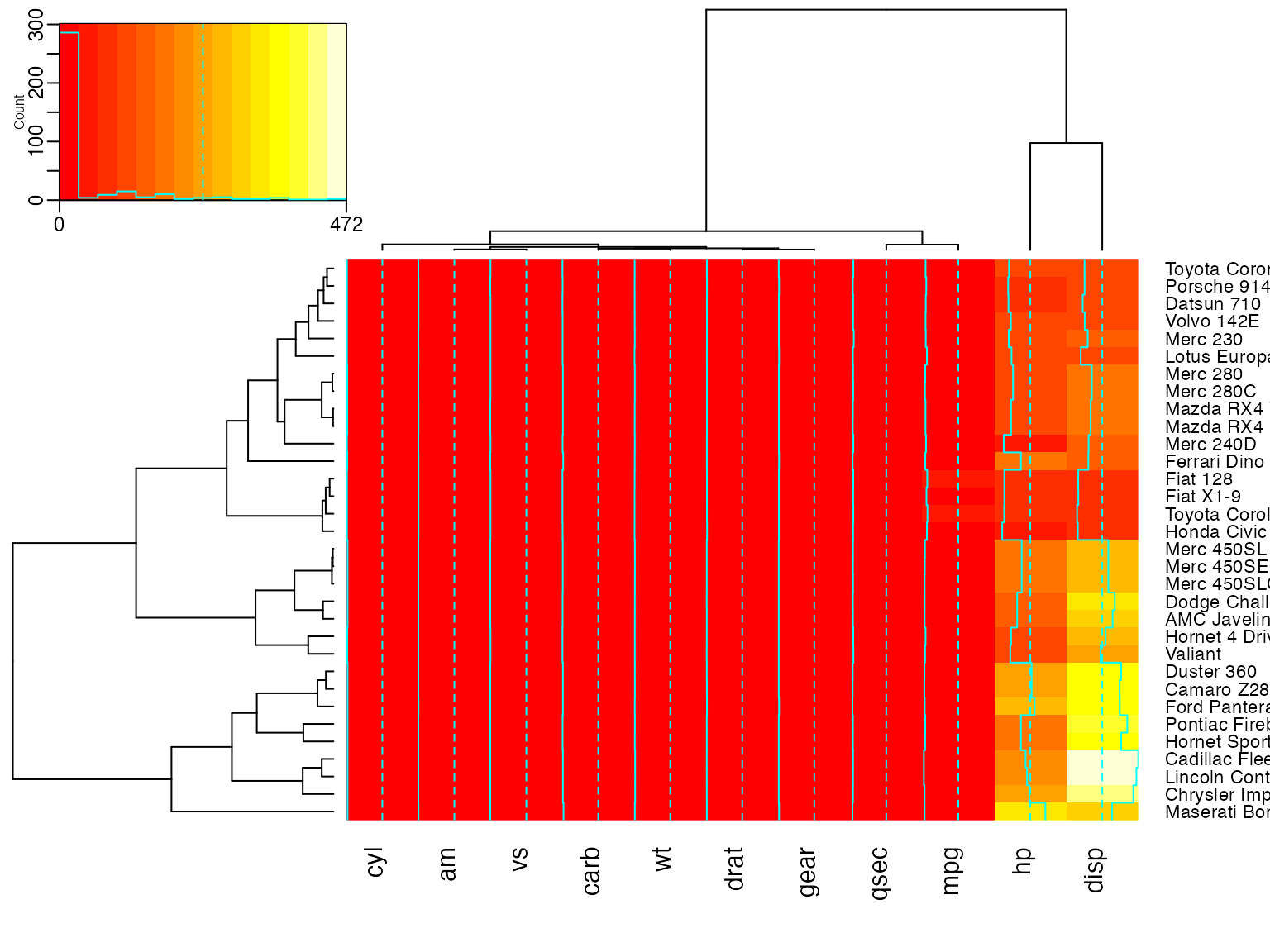
show how to customize the color key
heatmap.2(x,
         key.title=NA, # no title
         key.xlab=NA,  # no xlab
         key.par=list(mgp=c(1.5, 0.5, 0),
                      mar=c(2.5, 2.5, 1, 0)),
         key.xtickfun=function() {
               breaks <- parent.frame()$breaks
               return(list(
                    at=parent.frame()$scale01(c(breaks[1],
                                                breaks[length(breaks)])),
                    labels=c(as.character(breaks[1]),
                             as.character(breaks[length(breaks)]))
                    ))
         })
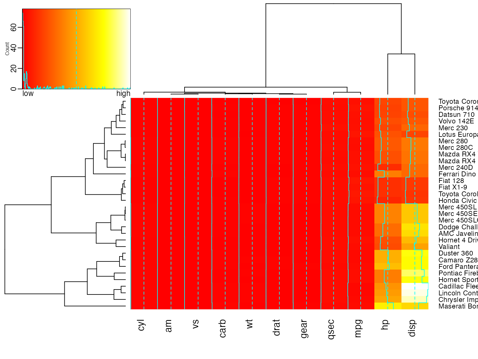
heatmap.2(x,
        breaks=256,
        key.title=NA,
        key.xlab=NA,
        key.par=list(mgp=c(1.5, 0.5, 0),
                     mar=c(1, 2.5, 1, 0)),
        key.xtickfun=function() {
             cex <- par("cex")*par("cex.axis")
             side <- 1
             line <- 0
             col <- par("col.axis")
             font <- par("font.axis")
             mtext("low", side=side, at=0, adj=0,
                   line=line, cex=cex, col=col, font=font)
             mtext("high", side=side, at=1, adj=1,
                   line=line, cex=cex, col=col, font=font)
             return(list(labels=FALSE, tick=FALSE))
        })
Show effect of z-score scaling within columns, blue-red color scale
##
##
hv <- heatmap.2(x, col=bluered, scale="column", tracecol="#303030")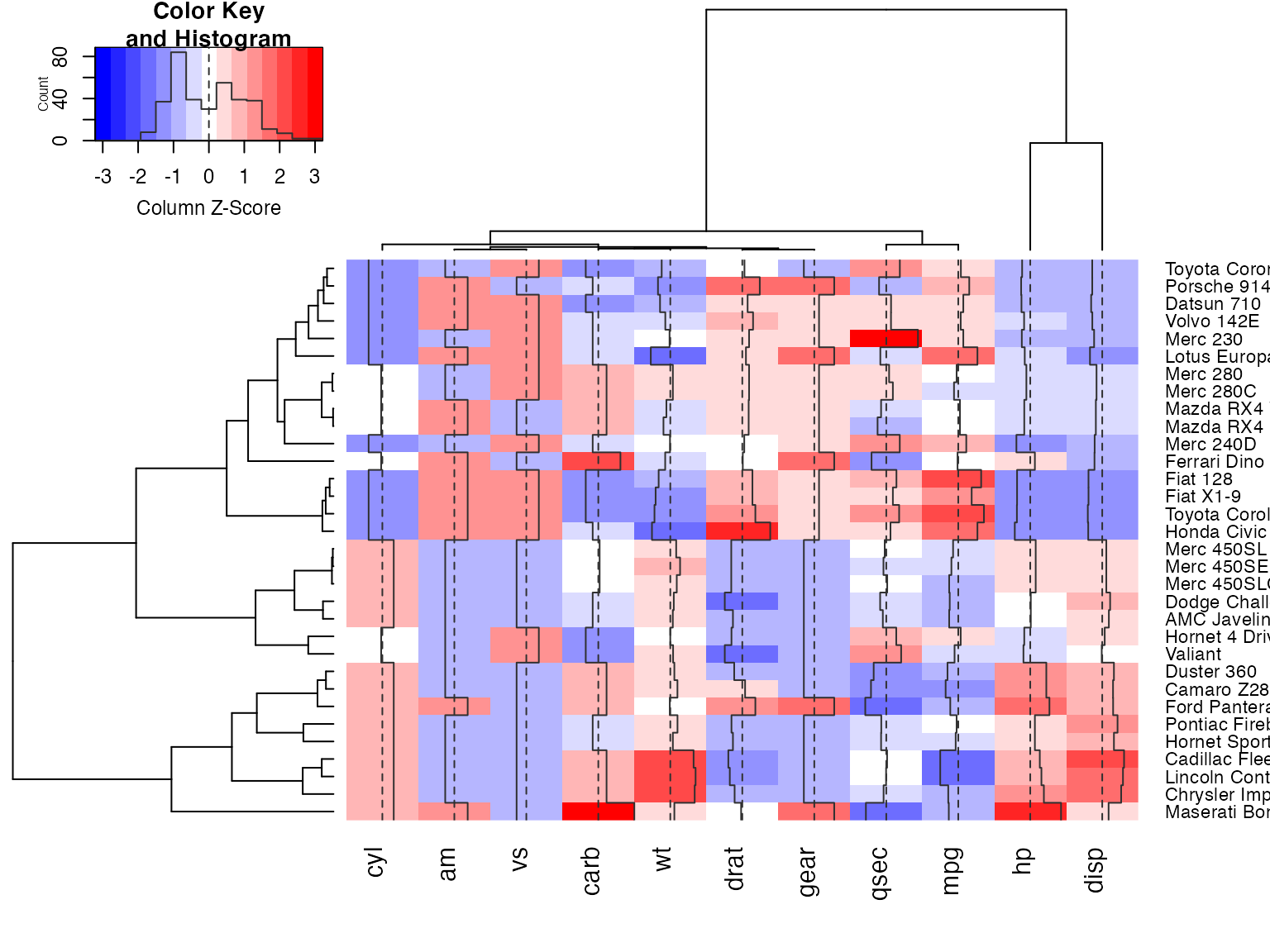
###
## Look at the return values
###
names(hv)
## [1] "rowInd" "colInd" "call" "colMeans"
## [5] "colSDs" "carpet" "rowDendrogram" "colDendrogram"
## [9] "breaks" "col" "vline" "colorTable"
## [13] "layout"
## Show the mapping of z-score values to color bins
hv$colorTable
## low high color
## 1 -3.2116766 -2.7834531 #0000FF
## 2 -2.7834531 -2.3552295 #2424FF
## 3 -2.3552295 -1.9270060 #4949FF
## 4 -1.9270060 -1.4987824 #6D6DFF
## 5 -1.4987824 -1.0705589 #9292FF
## 6 -1.0705589 -0.6423353 #B6B6FF
## 7 -0.6423353 -0.2141118 #DBDBFF
## 8 -0.2141118 0.2141118 #FFFFFF
## 9 0.2141118 0.6423353 #FFDBDB
## 10 0.6423353 1.0705589 #FFB6B6
## 11 1.0705589 1.4987824 #FF9292
## 12 1.4987824 1.9270060 #FF6D6D
## 13 1.9270060 2.3552295 #FF4949
## 14 2.3552295 2.7834531 #FF2424
## 15 2.7834531 3.2116766 #FF0000
## Extract the range associated with white
hv$colorTable[hv$colorTable[,"color"]=="#FFFFFF",]
## low high color
## 8 -0.2141118 0.2141118 #FFFFFF
## Determine the original data values that map to white
whiteBin <- unlist(hv$colorTable[hv$colorTable[,"color"]=="#FFFFFF",1:2])
rbind(whiteBin[1] * hv$colSDs + hv$colMeans,
     whiteBin[2] * hv$colSDs + hv$colMeans )
## cyl am vs carb wt drat gear qsec
## [1,] 5.805113 0.2994102 0.3295842 2.466667 3.007751 3.482081 3.529527 17.46614
## [2,] 6.569887 0.5130898 0.5454158 3.158333 3.426749 3.711044 3.845473 18.23136
## mpg hp disp
## [1,] 18.80018 132.0074 204.1851
## [2,] 21.38107 161.3676 257.2586
##
## A more decorative heatmap, with z-score scaling along columns
##
hv <- heatmap.2(x, col=cm.colors(255), scale="column",
       RowSideColors=rc, ColSideColors=cc, margin=c(5, 10),
       xlab="specification variables", ylab= "Car Models",
       main="heatmap(<Mtcars data>, ..., scale=\"column\")",
       tracecol="green", density="density")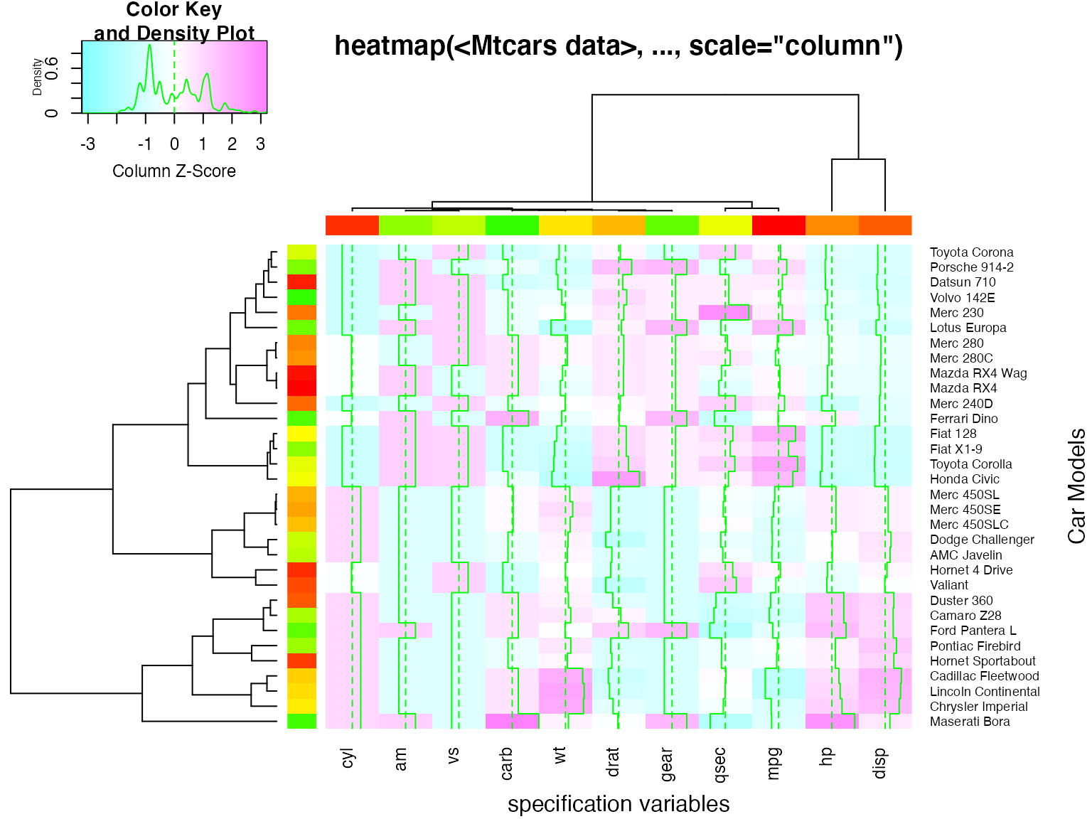
## Note that the breakpoints are now symmetric about 0

## Color the labels to match RowSideColors and ColSideColors
hv <- heatmap.2(x, col=cm.colors(255), scale="column",
       RowSideColors=rc, ColSideColors=cc, margin=c(5, 10),
       xlab="specification variables", ylab= "Car Models",
       main="heatmap(<Mtcars data>, ..., scale=\"column\")",
       tracecol="green", density="density", colRow=rc, colCol=cc,
       srtCol=45, adjCol=c(0.5,1))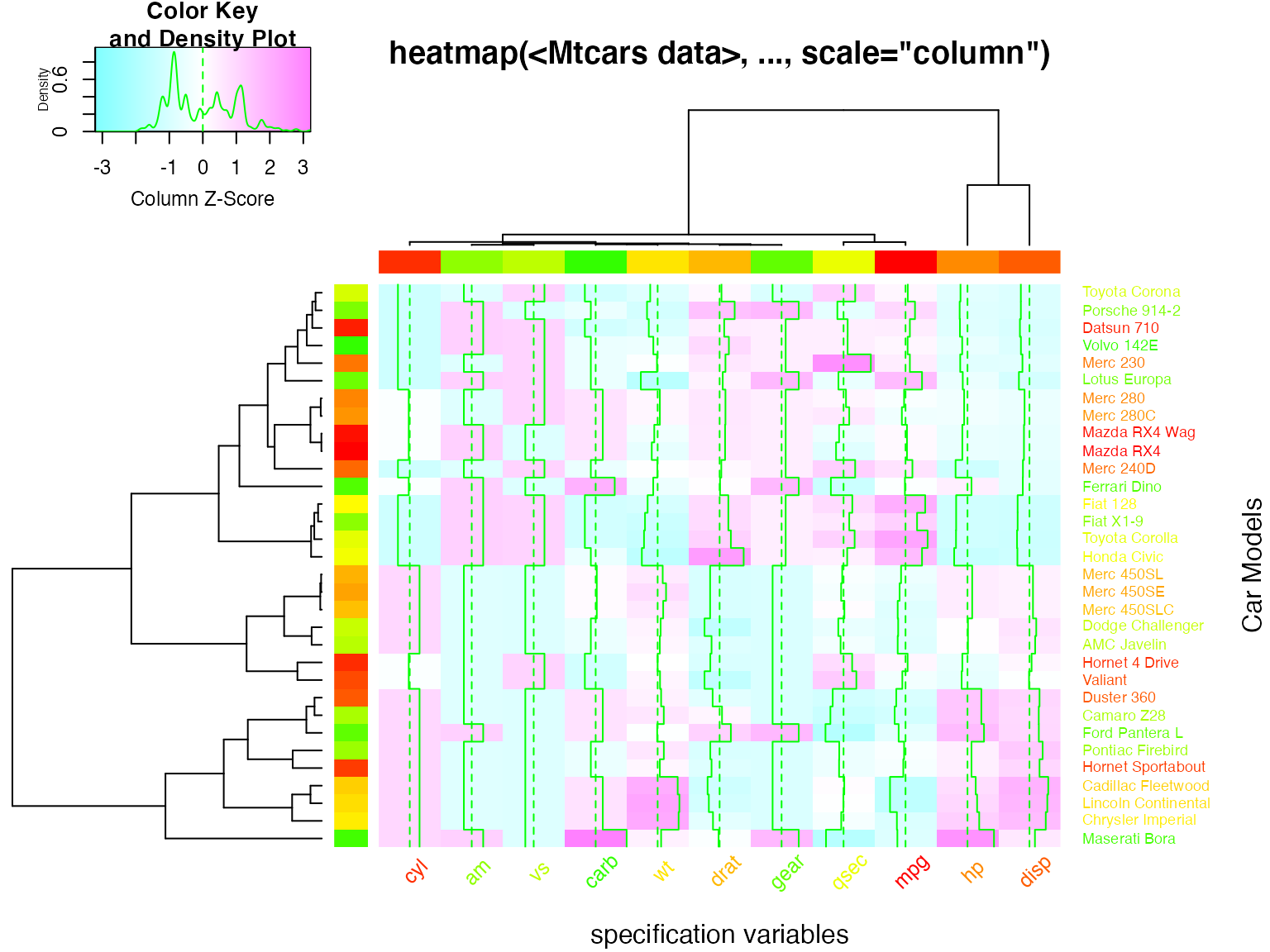
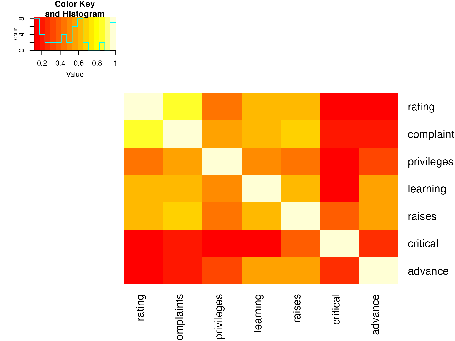
Correlation Heatmaps
##            rating complaints privileges learning raises critical advance
## rating       1.00       0.83       0.43     0.62   0.59     0.16    0.16
## complaints   0.83       1.00       0.56     0.60   0.67     0.19    0.22
## privileges   0.43       0.56       1.00     0.49   0.45     0.15    0.34
## learning     0.62       0.60       0.49     1.00   0.64     0.12    0.53
## raises       0.59       0.67       0.45     0.64   1.00     0.38    0.57
## critical     0.16       0.19       0.15     0.12   0.38     1.00    0.28
## advance      0.16       0.22       0.34     0.53   0.57     0.28    1.00
symnum(Ca) # simple graphic## rt cm p l rs cr a
## rating 1
## complaints + 1
## privileges . . 1
## learning , . . 1
## raises . , . , 1
## critical . 1
## advance . . . 1
## attr(,"legend")
## [1] 0 ' ' 0.3 '.' 0.6 ',' 0.8 '+' 0.9 '*' 0.95 'B' 1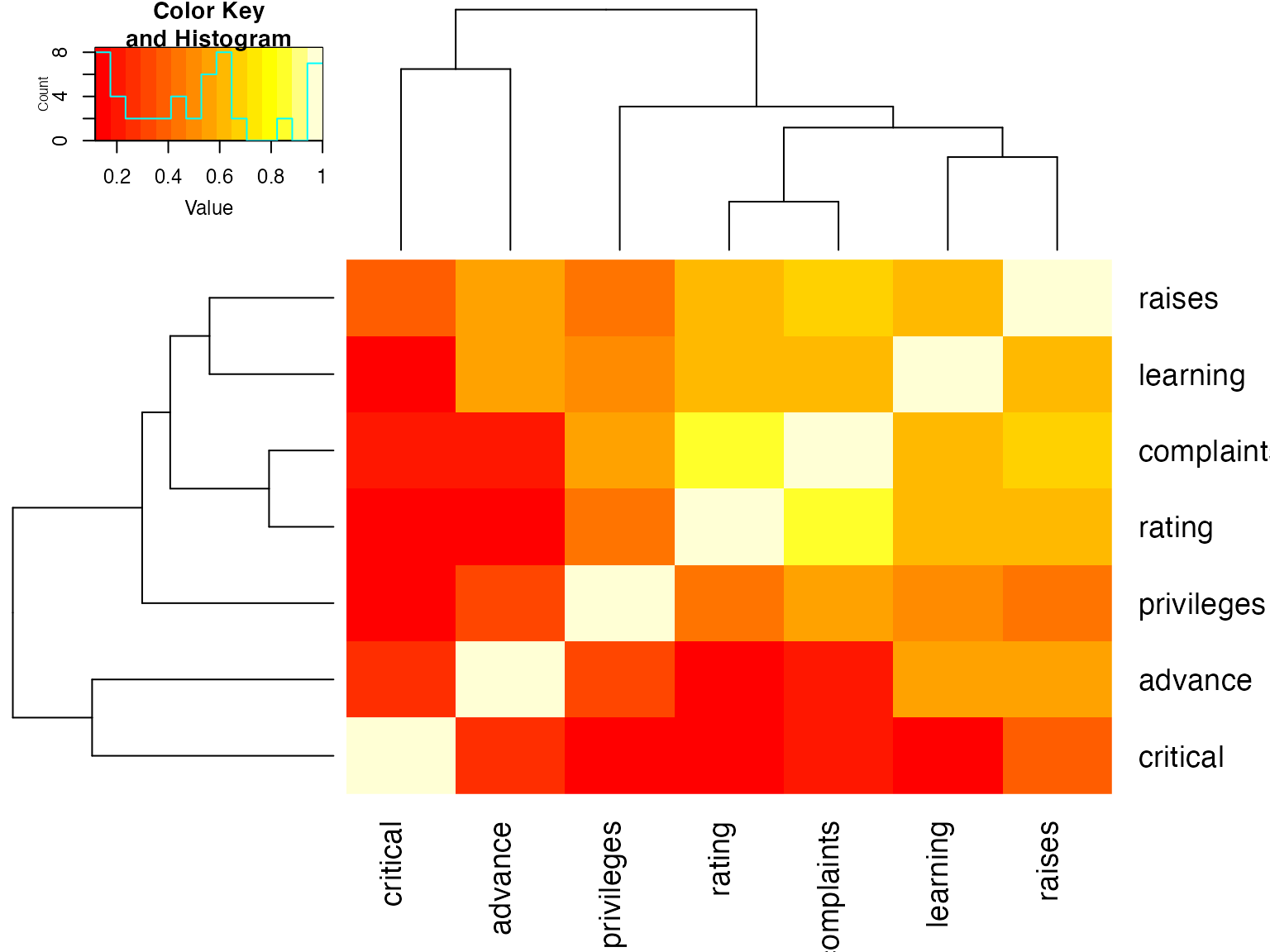
## Place the color key below the image plot
heatmap.2(x, lmat=rbind( c(0, 3), c(2,1), c(0,4) ), lhei=c(1.5, 4, 2 ) )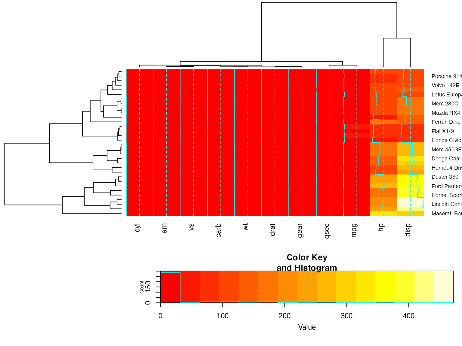
## Place the color key to the top right of the image plot
heatmap.2(x, lmat=rbind( c(0, 3, 4), c(2,1,0 ) ), lwid=c(1.5, 4, 2 ) )
For variable clustering, rather use distance based on cor():
##      CO I DM DI CF DE PR F O W PH R
## CONT 1
## INTG    1
## DMNR    B 1
## DILG    + +  1
## CFMG    + +  B  1
## DECI    + +  B  B  1
## PREP    + +  B  B  B  1
## FAMI    + +  B  *  *  B  1
## ORAL    * *  B  B  *  B  B 1
## WRIT    * +  B  *  *  B  B B 1
## PHYS    , ,  +  +  +  +  + + + 1
## RTEN    * *  *  *  *  B  * B B *  1
## attr(,"legend")
## [1] 0 ' ' 0.3 '.' 0.6 ',' 0.8 '+' 0.9 '*' 0.95 'B' 1
hU <- heatmap.2(cU, Rowv=FALSE, symm=TRUE, col=topo.colors(16),
            distfun=function(c) as.dist(1 - c), trace="none")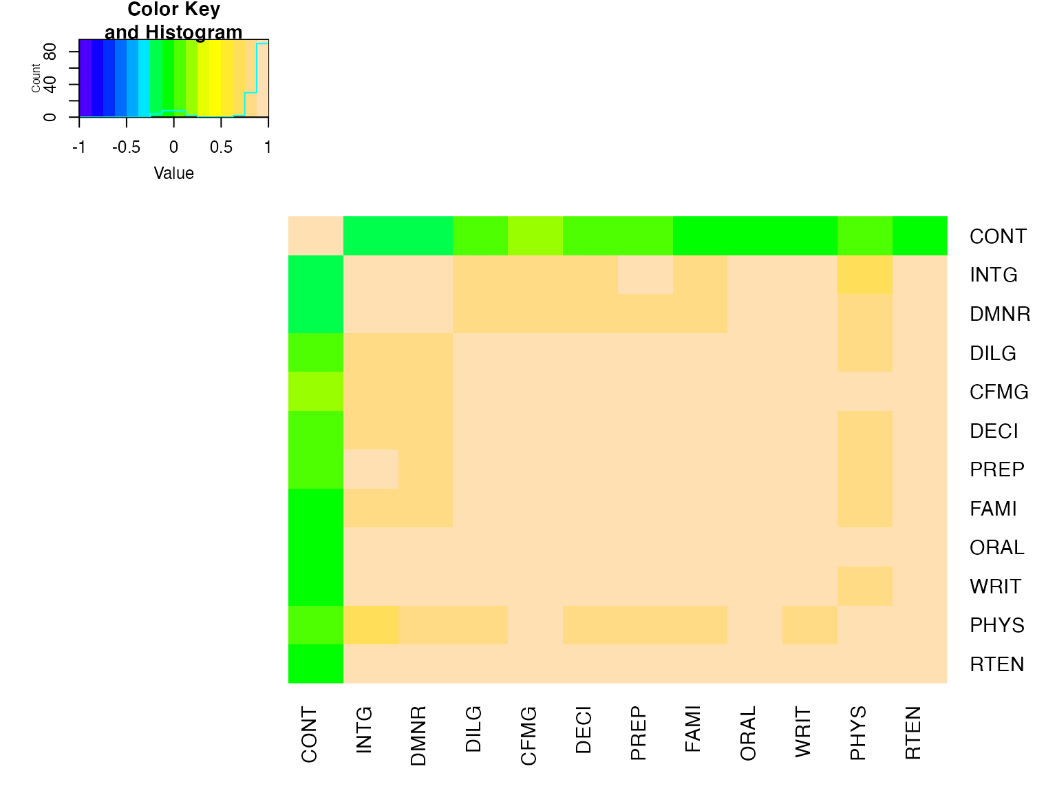
##      CONT    INTG    DMNR    DILG    CFMG    DECI    PREP    FAMI    ORAL
## CONT " 1.00" "-0.13" "-0.15" " 0.01" " 0.14" " 0.09" " 0.01" "-0.03" "-0.01"
## INTG "-0.13" " 1.00" " 0.96" " 0.87" " 0.81" " 0.80" " 0.88" " 0.87" " 0.91"
## DMNR "-0.15" " 0.96" " 1.00" " 0.84" " 0.81" " 0.80" " 0.86" " 0.84" " 0.91"
## DILG " 0.01" " 0.87" " 0.84" " 1.00" " 0.96" " 0.96" " 0.98" " 0.96" " 0.95"
## CFMG " 0.14" " 0.81" " 0.81" " 0.96" " 1.00" " 0.98" " 0.96" " 0.94" " 0.95"
## DECI " 0.09" " 0.80" " 0.80" " 0.96" " 0.98" " 1.00" " 0.96" " 0.94" " 0.95"
## PREP " 0.01" " 0.88" " 0.86" " 0.98" " 0.96" " 0.96" " 1.00" " 0.99" " 0.98"
## FAMI "-0.03" " 0.87" " 0.84" " 0.96" " 0.94" " 0.94" " 0.99" " 1.00" " 0.98"
## ORAL "-0.01" " 0.91" " 0.91" " 0.95" " 0.95" " 0.95" " 0.98" " 0.98" " 1.00"
## WRIT "-0.04" " 0.91" " 0.89" " 0.96" " 0.94" " 0.95" " 0.99" " 0.99" " 0.99"
## PHYS " 0.05" " 0.74" " 0.79" " 0.81" " 0.88" " 0.87" " 0.85" " 0.84" " 0.89"
## RTEN "-0.03" " 0.94" " 0.94" " 0.93" " 0.93" " 0.92" " 0.95" " 0.94" " 0.98"
##      WRIT    PHYS    RTEN
## CONT "-0.04" " 0.05" "-0.03"
## INTG " 0.91" " 0.74" " 0.94"
## DMNR " 0.89" " 0.79" " 0.94"
## DILG " 0.96" " 0.81" " 0.93"
## CFMG " 0.94" " 0.88" " 0.93"
## DECI " 0.95" " 0.87" " 0.92"
## PREP " 0.99" " 0.85" " 0.95"
## FAMI " 0.99" " 0.84" " 0.94"
## ORAL " 0.99" " 0.89" " 0.98"
## WRIT " 1.00" " 0.86" " 0.97"
## PHYS " 0.86" " 1.00" " 0.91"
## RTEN " 0.97" " 0.91" " 1.00"
now with the correlation matrix on the plot itself
heatmap.2(cU, Rowv=FALSE, symm=TRUE, col=rev(heat.colors(16)),
           distfun=function(c) as.dist(1 - c), trace="none",
           cellnote=hM)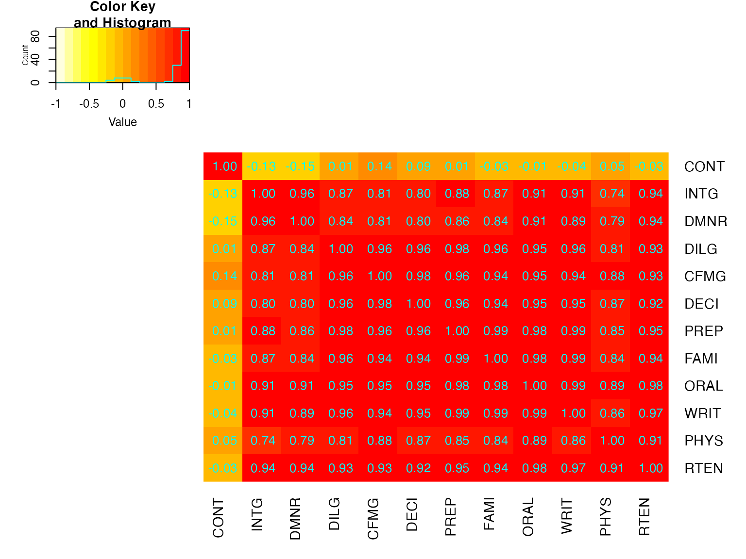
Interactive heatmap.2 using heatmaply
data(mtcars)
x  <- as.matrix(mtcars)

library(heatmaply)
# just use heatmaply instead of heatmap.2
heatmaply(x)
The default are slightly different, but it supports most of the same arguments. If you want the dendrograms to match perfectly, use this:
full <- heatmap.2(x) # we use it to easily get the dendrograms
## Color branches of dendrograms by cluster membership using dendextend:
heatmaply(x,
        Rowv=color_branches(full$rowDendrogram, k = 3),
        Colv=color_branches(full$colDendrogram, k = 2))
# Look at the vignette for more details:
# https://cran.r-project.org/web/packages/heatmaply/vignettes/heatmaply.html
Session Information
## R version 4.4.1 (2024-06-14)
## Platform: x86_64-apple-darwin20
## Running under: macOS Big Sur 11.7.10
##
## Matrix products: default
## BLAS:   /Library/Frameworks/R.framework/Versions/4.4-x86_64/Resources/lib/libRblas.0.dylib
## LAPACK: /Library/Frameworks/R.framework/Versions/4.4-x86_64/Resources/lib/libRlapack.dylib;  LAPACK version 3.12.0
##
## locale:
## [1] en_US.UTF-8/en_US.UTF-8/en_US.UTF-8/C/en_US.UTF-8/en_US.UTF-8
##
## time zone: Asia/Jerusalem
## tzcode source: internal
##
## attached base packages:
## [1] stats     graphics  grDevices utils     datasets  methods   base
##
## other attached packages:
## [1] heatmaply_1.6.0    viridis_0.6.5      viridisLite_0.4.2  plotly_4.10.4
## [5] ggplot2_3.5.1      dendextend_1.19.0  RColorBrewer_1.1-3 gplots_3.3.0
##
## loaded via a namespace (and not attached):
##  [1] gtable_0.3.5       xfun_0.47          bslib_0.8.0        htmlwidgets_1.6.4
##  [5] caTools_1.18.2     crosstalk_1.2.1    vctrs_0.6.5        tools_4.4.1
##  [9] bitops_1.0-8       generics_0.1.3     tibble_3.2.1       ca_0.71.1
## [13] fansi_1.0.6        highr_0.11         pkgconfig_2.0.3    KernSmooth_2.23-24
## [17] data.table_1.16.0  desc_1.4.3         assertthat_0.2.1   webshot_0.5.5
## [21] lifecycle_1.0.4    stringr_1.5.1      compiler_4.4.1     farver_2.1.2
## [25] textshaping_0.4.0  munsell_0.5.1      codetools_0.2-20   seriation_1.5.6
## [29] htmltools_0.5.8.1  sass_0.4.9         yaml_2.3.10        lazyeval_0.2.2
## [33] pillar_1.9.0       pkgdown_2.2.0      jquerylib_0.1.4    tidyr_1.3.1
## [37] cachem_1.1.0       iterators_1.0.14   TSP_1.2-4          foreach_1.5.2
## [41] gtools_3.9.5       tidyselect_1.2.1   digest_0.6.37      stringi_1.8.4
## [45] dplyr_1.1.4        reshape2_1.4.4     purrr_1.0.2        labeling_0.4.3
## [49] fastmap_1.2.0      grid_4.4.1         colorspace_2.1-1   cli_3.6.5
## [53] magrittr_2.0.3     utf8_1.2.4         withr_3.0.2        scales_1.3.0
## [57] registry_0.5-1     rmarkdown_2.28     httr_1.4.7         gridExtra_2.3
## [61] ragg_1.5.0         evaluate_1.0.5     knitr_1.48         rlang_1.1.6
## [65] Rcpp_1.0.13        glue_1.7.0         rstudioapi_0.16.0  jsonlite_1.8.8
## [69] R6_2.5.1           plyr_1.8.9         systemfonts_1.1.0  fs_1.6.6