Create 2-dimensional empirical confidence regions
ci2d.RdCreate 2-dimensional empirical confidence regions from provided data.
ci2d(x, y = NULL,
     nbins=51, method=c("bkde2D","hist2d"),
     bandwidth, factor=1.0,
     ci.levels=c(0.50,0.75,0.90,0.95,0.975),
     show=c("filled.contour","contour","image","none"),
     col=topo.colors(length(breaks)-1),
     show.points=FALSE,
     pch=par("pch"),
     points.col="red",
     xlab, ylab,
     ...)
# S3 method for class 'ci2d'
print(x, ...)
Arguments
- x
either a vector containing the x coordinates or a matrix with 2 columns.
- y
a vector contianing the y coordinates, not required if `x' is matrix
- nbins
number of bins in each dimension. May be a scalar or a 2 element vector. Defaults to 51.
- method
One of "bkde2D" (for KernSmooth::bdke2d) or "hist2d" (for gplots::hist2d) specifyting the name of the method to create the 2-d density summarizing the data. Defaults to "bkde2D".
- bandwidth
Bandwidth to use for
KernSmooth::bkde2D. See below for default value.- factor
Numeric scaling factor for bandwidth. Useful for exploring effect of changing the bandwidth. Defaults to 1.0.
- ci.levels
Confidence level(s) to use for plotting data. Defaults to
c(0.5, 0.75, 0.9, 0.95, 0.975)- show
Plot type to be displaed. One of "filled.contour", "contour", "image", or "none". Defaults to "filled.contour".
- show.points
Boolean indicating whether original data values should be plotted. Defaults to
TRUE.- pch
Point type for plots. See
pointsfor details.- points.col
Point color for plotting original data. Defaiults to "red".
- col
Colors to use for plots.
- xlab, ylab
Axis labels
- ...
Additional arguments passed to
KernSmooth::bkde2Dorgplots::hist2d.
Details
This function utilizes either KernSmooth::bkde2D or
gplots::hist2d to estmate a 2-dimensional density of the data
passed as an argument. This density is then used to create and
(optionally) display confidence regions.
When bandwidth is ommited and method="bkde2d",
KernSmooth::dpik is appled in x and y dimensions to select the
bandwidth.
Note
Confidence intervals generated by ci2d are approximate, and are subject to biases and/or artifacts induced by the binning or kernel smoothing method, bin locations, bin sizes, and kernel bandwidth.
The conf2d function in the r2d2 package may create a more
accurate confidence region, and reports the actual proportion of
points inside the region.
Value
A ci2d object consisting of a list containing (at least) the
following elements:
- nobs
number of original data points
- x
x position of each density estimate bin
- y
y position of each density estimate bin
- density
Matrix containing the probability density of each bin (count in bin/total count)
- cumDensity
Matrix where each element contains the cumulative probability density of all elements with the same density (used to create the confidence region plots)
- contours
List of contours of each confidence region.
- call
Call used to create this object
Examples
####
## Basic usage
####
data(geyser, package="MASS")
x <- geyser$duration
y <- geyser$waiting
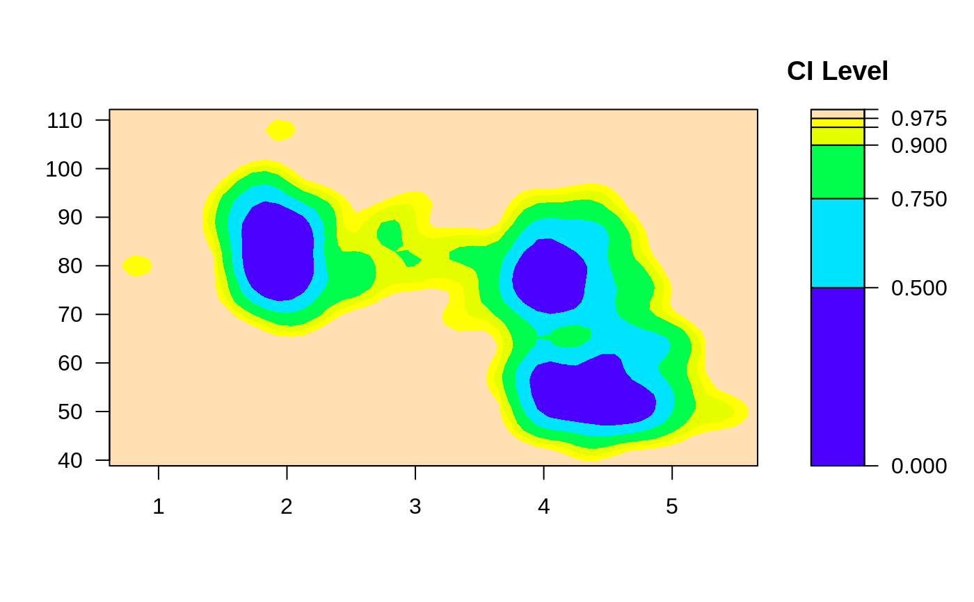
# 2-d confidence intervals based on binned kernel density estimate
ci2d(x,y) # filled contour plot
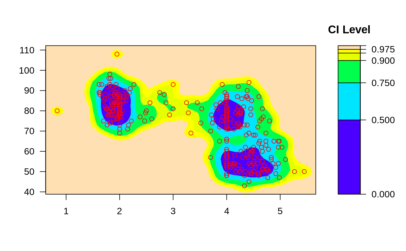
 ci2d(x,y, show.points=TRUE) # show original data
 # image plot
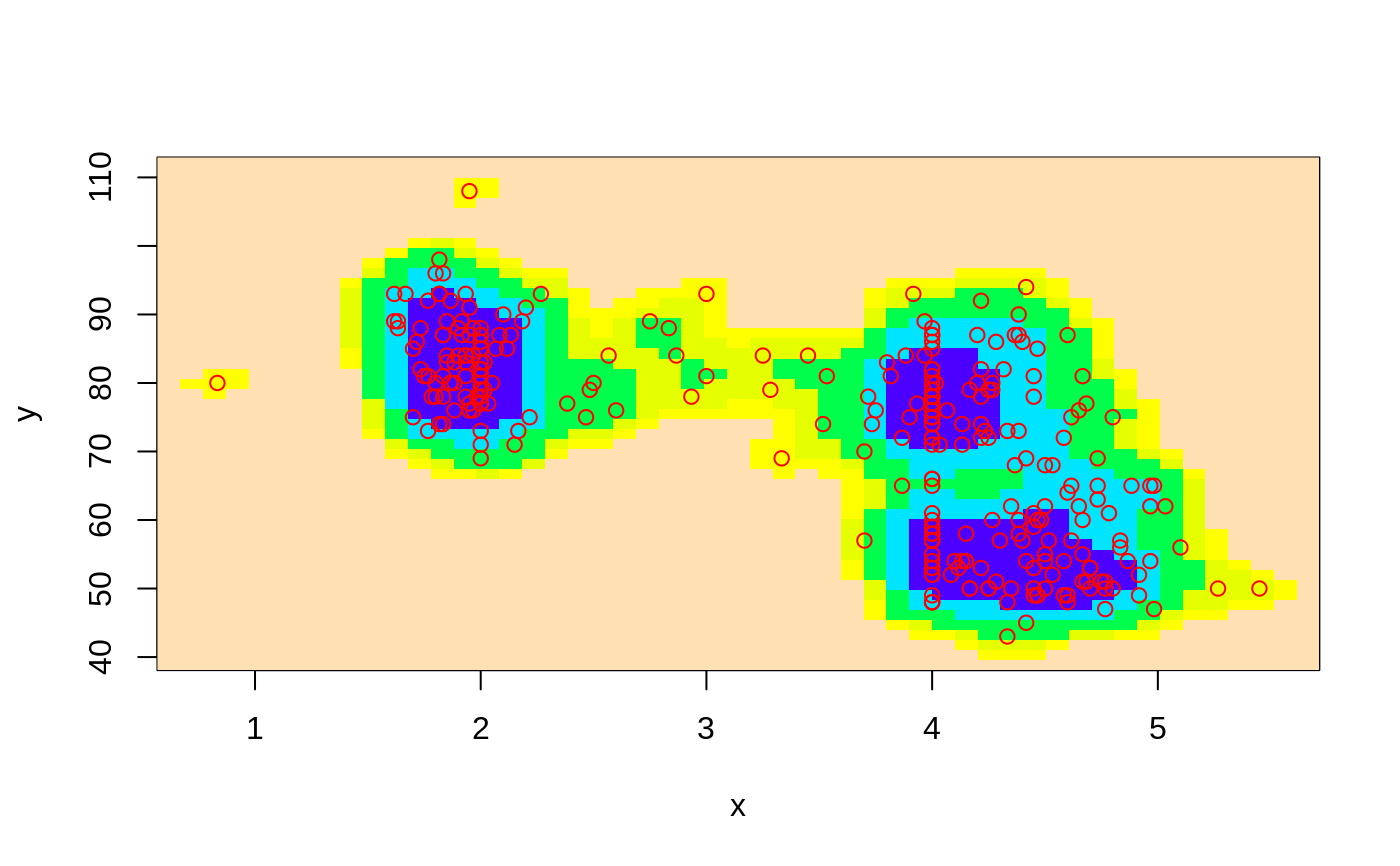
ci2d(x,y, show="image")
ci2d(x,y, show="image", show.points=TRUE)
# image plot
ci2d(x,y, show="image")
ci2d(x,y, show="image", show.points=TRUE)
 # contour plot
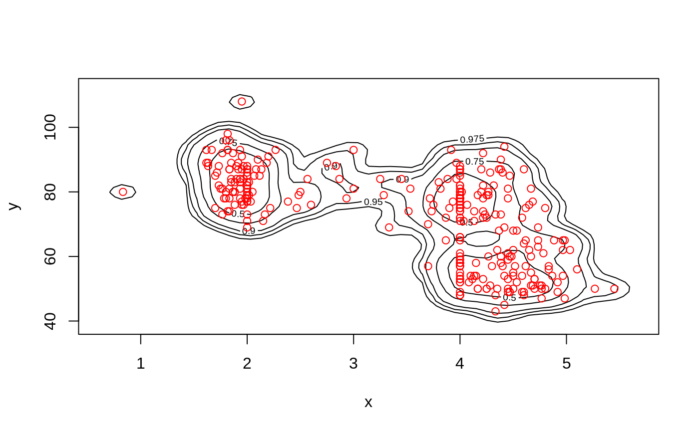
ci2d(x,y, show="contour", col="black")
ci2d(x,y, show="contour", col="black", show.points=TRUE)
# contour plot
ci2d(x,y, show="contour", col="black")
ci2d(x,y, show="contour", col="black", show.points=TRUE)
 ####
## Control Axis scales
####
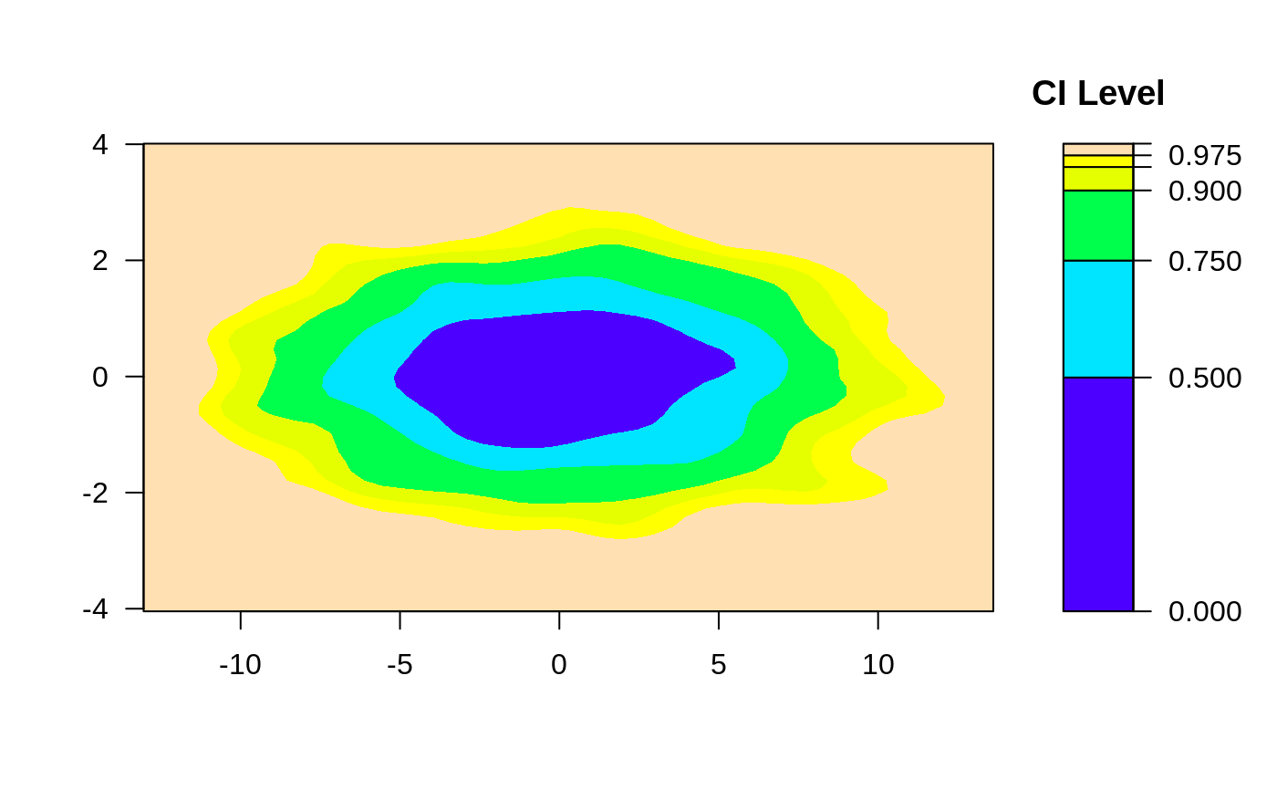
x <- rnorm(2000, sd=4)
y <- rnorm(2000, sd=1)
# 2-d confidence intervals based on binned kernel density estimate
ci2d(x,y)
####
## Control Axis scales
####
x <- rnorm(2000, sd=4)
y <- rnorm(2000, sd=1)
# 2-d confidence intervals based on binned kernel density estimate
ci2d(x,y)
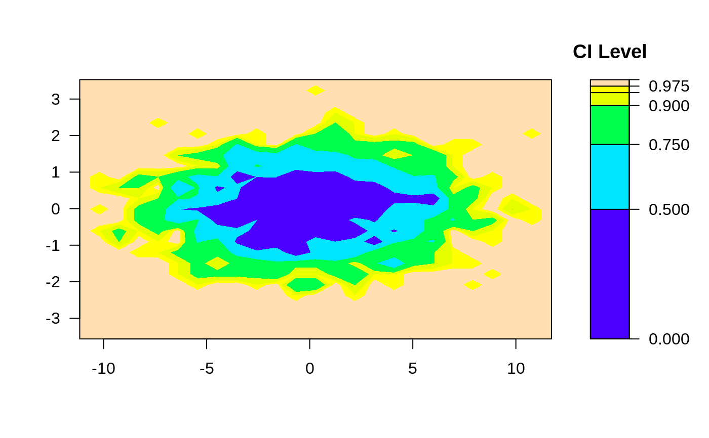
 # 2-d confidence intervals based on 2d histogram
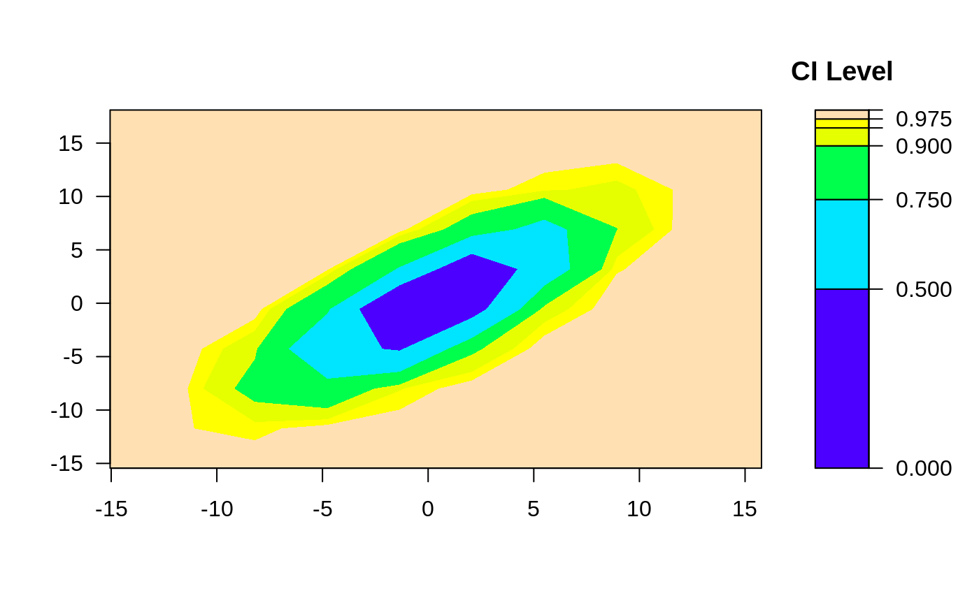
ci2d(x,y, method="hist2d", nbins=25)
# 2-d confidence intervals based on 2d histogram
ci2d(x,y, method="hist2d", nbins=25)
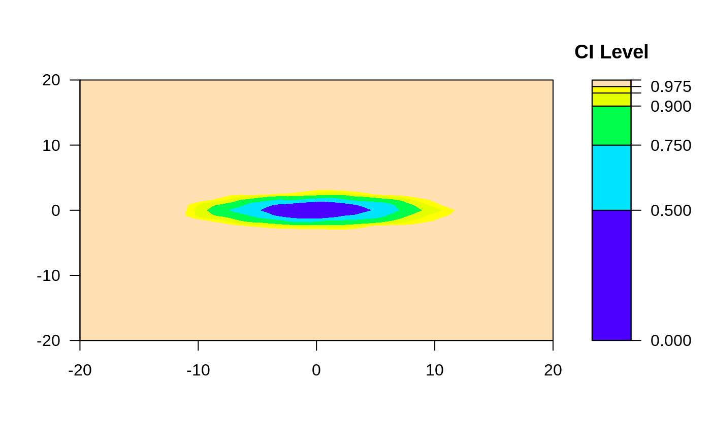
 # Require same scale for each axis, this looks oval
ci2d(x,y, range.x=list(c(-20,20), c(-20,20)))
#> Warning: Binning grid too coarse for current (small) bandwidth: consider increasing 'gridsize'
# Require same scale for each axis, this looks oval
ci2d(x,y, range.x=list(c(-20,20), c(-20,20)))
#> Warning: Binning grid too coarse for current (small) bandwidth: consider increasing 'gridsize'
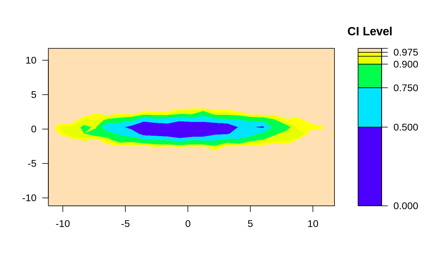
 ci2d(x,y, method="hist2d", same.scale=TRUE, nbins=25) # hist2d
 ####
## Control smoothing and binning
####
x <- rnorm(2000, sd=4)
y <- rnorm(2000, mean=x, sd=2)
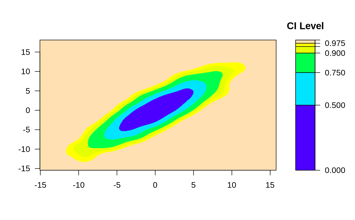
# Default 2-d confidence intervals based on binned kernel density estimate
ci2d(x,y)
####
## Control smoothing and binning
####
x <- rnorm(2000, sd=4)
y <- rnorm(2000, mean=x, sd=2)
# Default 2-d confidence intervals based on binned kernel density estimate
ci2d(x,y)
 # change the smoother bandwidth
ci2d(x,y,
bandwidth=c(sd(x)/8, sd(y)/8)
)
# change the smoother bandwidth
ci2d(x,y,
bandwidth=c(sd(x)/8, sd(y)/8)
)
 # change the smoother number of bins
ci2d(x,y, nbins=10)
#> Warning: Binning grid too coarse for current (small) bandwidth: consider increasing 'gridsize'
# change the smoother number of bins
ci2d(x,y, nbins=10)
#> Warning: Binning grid too coarse for current (small) bandwidth: consider increasing 'gridsize'
 ci2d(x,y)
 ci2d(x,y, nbins=100)
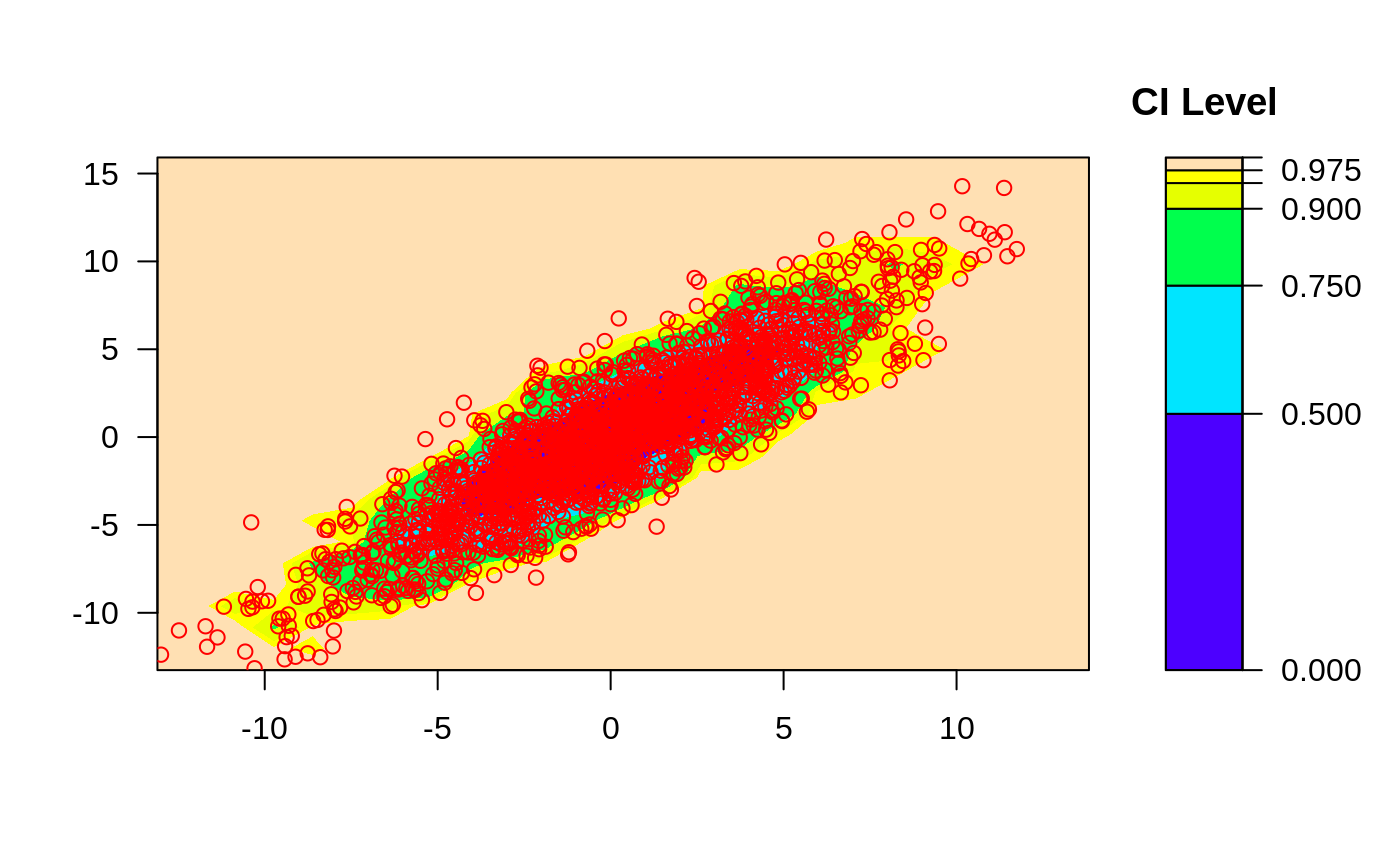
 # Default 2-d confidence intervals based on 2d histogram
ci2d(x,y, method="hist2d", show.points=TRUE)
# Default 2-d confidence intervals based on 2d histogram
ci2d(x,y, method="hist2d", show.points=TRUE)
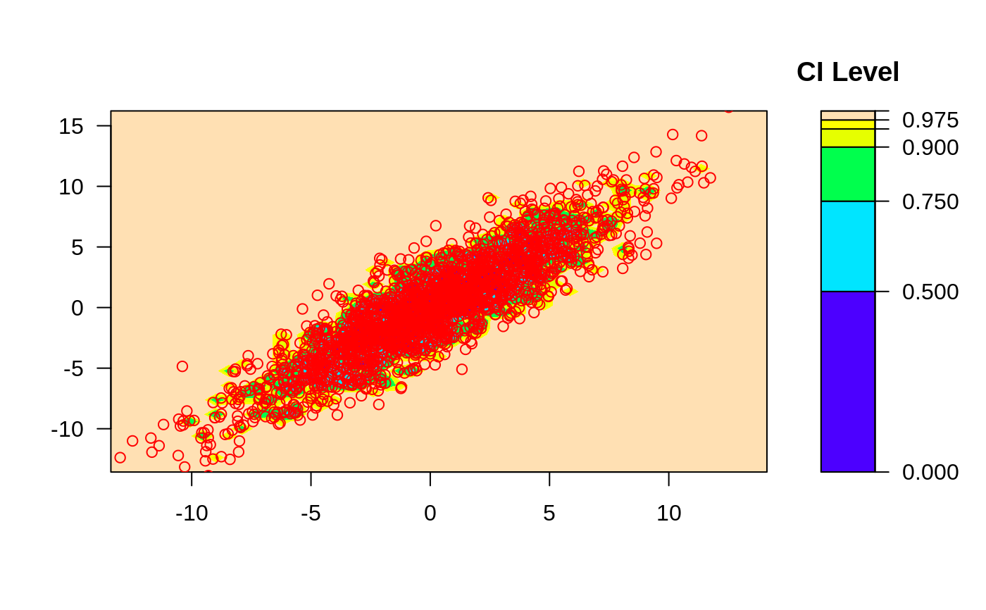 # change the number of histogram bins
ci2d(x,y, nbin=10, method="hist2d", show.points=TRUE )
# change the number of histogram bins
ci2d(x,y, nbin=10, method="hist2d", show.points=TRUE )
 ci2d(x,y, nbin=25, method="hist2d", show.points=TRUE )
 ####
## Perform plotting manually
####
data(geyser, package="MASS")
# let ci2d handle plotting contours...
ci2d(geyser$duration, geyser$waiting, show="contour", col="black")
####
## Perform plotting manually
####
data(geyser, package="MASS")
# let ci2d handle plotting contours...
ci2d(geyser$duration, geyser$waiting, show="contour", col="black")
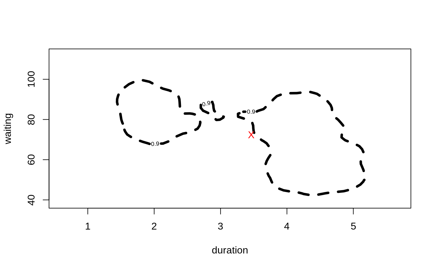
 # call contour() directly, show the 90 percent CI, and the mean point
est <- ci2d(geyser$duration, geyser$waiting, show="none")
contour(est$x, est$y, est$cumDensity,
xlab="duration", ylab="waiting",
levels=0.90, lwd=4, lty=2)
points(mean(geyser$duration), mean(geyser$waiting),
col="red", pch="X")
# call contour() directly, show the 90 percent CI, and the mean point
est <- ci2d(geyser$duration, geyser$waiting, show="none")
contour(est$x, est$y, est$cumDensity,
xlab="duration", ylab="waiting",
levels=0.90, lwd=4, lty=2)
points(mean(geyser$duration), mean(geyser$waiting),
col="red", pch="X")
 ####
## Extract confidence region values
###
data(geyser, package="MASS")
## Empirical 90 percent confidence limits
quantile( geyser$duration, c(0.05, 0.95) )
#> 5% 95%
#> 1.781667 4.803333
quantile( geyser$waiting, c(0.05, 0.95) )
#> 5% 95%
#> 49 92
## Bivariate 90 percent confidence region
est <- ci2d(geyser$duration, geyser$waiting, show="none")
names(est$contours) ## show available contours
#> [1] "0.5" "0.5" "0.5" "0.75" "0.75" "0.9" "0.9" "0.9" "0.95"
#> [10] "0.975" "0.975" "0.975" "1" "1" "1" "1"
ci.90 <- est$contours[names(est$contours)=="0.9"] # get region(s)
ci.90 <- rbind(ci.90[[1]],NA, ci.90[[2]], NA, ci.90[[3]]) # join them
print(ci.90) # show full contour
#> x y
#> 1 1.526652 78.00100
#> 2 1.520334 78.43451
#> 3 1.505526 79.90177
#> 4 1.498197 81.36902
#> 5 1.490886 82.83628
#> 6 1.479440 84.30353
#> 7 1.462897 85.77079
#> 8 1.449958 87.23804
#> 9 1.440848 88.70530
#> 10 1.442839 90.17255
#> 11 1.454784 91.63981
#> 12 1.472003 93.10706
#> 13 1.500685 94.57432
#> 14 1.526652 95.19393
#> 15 1.559131 96.04157
#> 16 1.617806 97.50883
#> 17 1.627590 97.68333
#> 18 1.714635 98.97608
#> 19 1.728529 99.16754
#> 20 1.829467 99.52422
#> 21 1.902190 98.97608
#> 22 1.930405 98.75198
#> 23 2.001441 97.50883
#> 24 2.031344 96.96819
#> 25 2.085418 96.04157
#> 26 2.132282 95.33502
#> 27 2.215860 94.57432
#> 28 2.233221 94.38900
#> 29 2.317325 93.10706
#> 30 2.334159 92.65774
#> 31 2.364668 91.63981
#> 32 2.379204 90.17255
#> 33 2.383578 88.70530
#> 34 2.386307 87.23804
#> 35 2.388831 85.77079
#> 36 2.399318 84.30353
#> 37 2.435098 82.94130
#> 38 2.536036 83.00782
#> 39 2.576349 82.83628
#> 40 2.636974 82.27676
#> 41 2.667152 81.36902
#> 42 2.688972 79.90177
#> 43 2.694766 78.43451
#> 44 2.684505 76.96726
#> 45 2.655260 75.50000
#> 46 2.636974 75.15474
#> 47 2.569526 74.03274
#> 48 2.536036 73.63059
#> 49 2.435098 72.97800
#> 50 2.405518 72.56549
#> 51 2.334159 71.55041
#> 52 2.313730 71.09823
#> 53 2.251786 69.63098
#> 54 2.233221 69.32254
#> 55 2.142469 68.16372
#> 56 2.132282 68.03823
#> 57 2.031344 67.61998
#> 58 1.930405 67.86785
#> 59 1.904180 68.16372
#> 60 1.829467 68.88220
#> 61 1.764631 69.63098
#> 62 1.728529 70.03697
#> 63 1.661616 71.09823
#> 64 1.627590 71.79147
#> 65 1.592978 72.56549
#> 66 1.562754 74.03274
#> 67 1.543863 75.50000
#> 68 1.533815 76.96726
#> 69 1.526652 78.00100
#> 70 NA NA
#> 71 2.737913 84.36406
#> 72 2.702601 85.77079
#> 73 2.702726 87.23804
#> 74 2.728780 88.70530
#> 75 2.737913 88.92268
#> 76 2.838851 89.49949
#> 77 2.874943 88.70530
#> 78 2.890153 87.23804
#> 79 2.894175 85.77079
#> 80 2.904096 84.30353
#> 81 2.939790 83.29632
#> 82 2.956368 82.83628
#> 83 3.040728 81.45426
#> 84 3.047848 81.36902
#> 85 3.040728 80.91434
#> 86 2.988633 79.90177
#> 87 2.939790 79.77276
#> 88 2.931426 79.90177
#> 89 2.897488 81.36902
#> 90 2.841431 82.83628
#> 91 2.838851 82.84583
#> 92 2.742613 84.30353
#> 93 2.737913 84.36406
#> 94 NA NA
#> 95 3.343544 80.55432
#> 96 3.264362 81.36902
#> 97 3.262814 82.83628
#> 98 3.343544 83.86099
#> 99 3.444482 84.13361
#> 100 3.545420 83.98935
#> 101 3.564810 84.30353
#> 102 3.646359 85.16856
#> 103 3.667276 85.77079
#> 104 3.711371 87.23804
#> 105 3.747297 88.21581
#> 106 3.761295 88.70530
#> 107 3.799563 90.17255
#> 108 3.848236 91.61093
#> 109 3.850149 91.63981
#> 110 3.949174 92.85127
#> 111 4.050113 93.07323
#> 112 4.129626 93.10706
#> 113 4.151051 93.11728
#> 114 4.251989 93.52810
#> 115 4.352928 93.67499
#> 116 4.417983 93.10706
#> 117 4.453866 92.74089
#> 118 4.504468 91.63981
#> 119 4.554805 90.67480
#> 120 4.577976 90.17255
#> 121 4.620989 88.70530
#> 122 4.655743 87.29638
#> 123 4.657465 87.23804
#> 124 4.675729 85.77079
#> 125 4.679825 84.30353
#> 126 4.688109 82.83628
#> 127 4.713564 81.36902
#> 128 4.756682 80.27291
#> 129 4.770533 79.90177
#> 130 4.810875 78.43451
#> 131 4.847559 76.96726
#> 132 4.857620 76.04432
#> 133 4.863988 75.50000
#> 134 4.857620 74.76464
#> 135 4.851404 74.03274
#> 136 4.826268 72.56549
#> 137 4.822707 71.09823
#> 138 4.857620 70.14403
#> 139 4.879648 69.63098
#> 140 4.958558 68.64356
#> 141 4.993910 68.16372
#> 142 5.059497 67.26021
#> 143 5.091469 66.69647
#> 144 5.131592 65.22921
#> 145 5.151538 63.76196
#> 146 5.147964 62.29470
#> 147 5.130174 60.82745
#> 148 5.111120 59.36019
#> 149 5.113432 57.89294
#> 150 5.132810 56.42568
#> 151 5.151330 54.95843
#> 152 5.160435 53.90290
#> 153 5.165968 53.49117
#> 154 5.181295 52.02392
#> 155 5.186603 50.55666
#> 156 5.160435 49.79061
#> 157 5.149455 49.08941
#> 158 5.106121 47.62215
#> 159 5.059497 46.71834
#> 160 5.031109 46.15490
#> 161 4.958558 45.21630
#> 162 4.899437 44.68764
#> 163 4.857620 44.34279
#> 164 4.756682 43.99259
#> 165 4.655743 43.69261
#> 166 4.564788 43.22039
#> 167 4.554805 43.13902
#> 168 4.453866 42.53020
#> 169 4.352928 42.38644
#> 170 4.251989 42.94142
#> 171 4.227531 43.22039
#> 172 4.151051 43.84742
#> 173 4.050113 44.17547
#> 174 3.960667 44.68764
#> 175 3.949174 44.74952
#> 176 3.848236 46.03264
#> 177 3.841648 46.15490
#> 178 3.793690 47.62215
#> 179 3.769244 49.08941
#> 180 3.750798 50.55666
#> 181 3.747297 50.87603
#> 182 3.724850 52.02392
#> 183 3.705749 53.49117
#> 184 3.688124 54.95843
#> 185 3.677953 56.42568
#> 186 3.679643 57.89294
#> 187 3.695465 59.36019
#> 188 3.720085 60.82745
#> 189 3.747297 62.17827
#> 190 3.749205 62.29470
#> 191 3.761016 63.76196
#> 192 3.752194 65.22921
#> 193 3.747297 65.55238
#> 194 3.726328 66.69647
#> 195 3.693492 68.16372
#> 196 3.646359 69.23910
#> 197 3.623416 69.63098
#> 198 3.567201 71.09823
#> 199 3.545420 71.72056
#> 200 3.514052 72.56549
#> 201 3.499421 74.03274
#> 202 3.493647 75.50000
#> 203 3.491131 76.96726
#> 204 3.476675 78.43451
#> 205 3.444482 79.45455
#> 206 3.401653 79.90177
#> 207 3.343544 80.55432
range(ci.90$x, na.rm=TRUE) # range for duration
#> [1] 1.440848 5.186603
range(ci.90$y, na.rm=TRUE) # range for waiting
#> [1] 42.38644 99.52422
####
## Visually compare confidence regions
####
data(geyser, package="MASS")
## Bivariate smoothed 90 percent confidence region
est <- ci2d(geyser$duration, geyser$waiting, show="none")
names(est$contours) ## show available contours
#> [1] "0.5" "0.5" "0.5" "0.75" "0.75" "0.9" "0.9" "0.9" "0.95"
#> [10] "0.975" "0.975" "0.975" "1" "1" "1" "1"
ci.90 <- est$contours[names(est$contours)=="0.9"] # get region(s)
ci.90 <- rbind(ci.90[[1]],NA, ci.90[[2]], NA, ci.90[[3]]) # join them
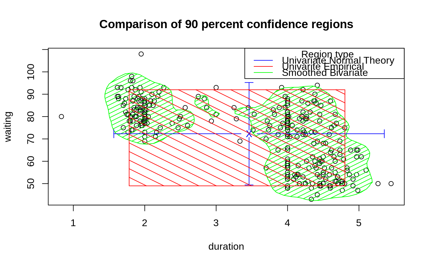
plot( waiting ~ duration, data=geyser,
main="Comparison of 90 percent confidence regions" )
polygon( ci.90, col="green", border="green", density=10)
## Univariate Normal-Theory 90 percent confidence region
mean.x <- mean(geyser$duration)
mean.y <- mean(geyser$waiting)
sd.x <- sd(geyser$duration)
sd.y <- sd(geyser$waiting)
t.value <- qt(c(0.05,0.95), df=length(geyser$duration), lower=TRUE)
ci.x <- mean.x + t.value* sd.x
ci.y <- mean.y + t.value* sd.y
plotCI(mean.x, mean.y,
li=ci.x[1],
ui=ci.x[2],
barcol="blue", col="blue",
err="x",
pch="X",
add=TRUE )
plotCI(mean.x, mean.y,
li=ci.y[1],
ui=ci.y[2],
barcol="blue", col="blue",
err="y",
pch=NA,
add=TRUE )
# rect(ci.x[1], ci.y[1], ci.x[2], ci.y[2], border="blue",
# density=5,
# angle=45,
# col="blue" )
## Empirical univariate 90 percent confidence region
box <- cbind( x=quantile( geyser$duration, c(0.05, 0.95 )),
y=quantile( geyser$waiting, c(0.05, 0.95 )) )
rect(box[1,1], box[1,2], box[2,1], box[2,2], border="red",
density=5,
angle=-45,
col="red" )
## now a nice legend
legend( "topright", legend=c(" Region type",
"Univariate Normal Theory",
"Univarite Empirical",
"Smoothed Bivariate"),
lwd=c(NA,1,1,1),
col=c("black","blue","red","green"),
lty=c(NA,1,1,1)
)
####
## Extract confidence region values
###
data(geyser, package="MASS")
## Empirical 90 percent confidence limits
quantile( geyser$duration, c(0.05, 0.95) )
#> 5% 95%
#> 1.781667 4.803333
quantile( geyser$waiting, c(0.05, 0.95) )
#> 5% 95%
#> 49 92
## Bivariate 90 percent confidence region
est <- ci2d(geyser$duration, geyser$waiting, show="none")
names(est$contours) ## show available contours
#> [1] "0.5" "0.5" "0.5" "0.75" "0.75" "0.9" "0.9" "0.9" "0.95"
#> [10] "0.975" "0.975" "0.975" "1" "1" "1" "1"
ci.90 <- est$contours[names(est$contours)=="0.9"] # get region(s)
ci.90 <- rbind(ci.90[[1]],NA, ci.90[[2]], NA, ci.90[[3]]) # join them
print(ci.90) # show full contour
#> x y
#> 1 1.526652 78.00100
#> 2 1.520334 78.43451
#> 3 1.505526 79.90177
#> 4 1.498197 81.36902
#> 5 1.490886 82.83628
#> 6 1.479440 84.30353
#> 7 1.462897 85.77079
#> 8 1.449958 87.23804
#> 9 1.440848 88.70530
#> 10 1.442839 90.17255
#> 11 1.454784 91.63981
#> 12 1.472003 93.10706
#> 13 1.500685 94.57432
#> 14 1.526652 95.19393
#> 15 1.559131 96.04157
#> 16 1.617806 97.50883
#> 17 1.627590 97.68333
#> 18 1.714635 98.97608
#> 19 1.728529 99.16754
#> 20 1.829467 99.52422
#> 21 1.902190 98.97608
#> 22 1.930405 98.75198
#> 23 2.001441 97.50883
#> 24 2.031344 96.96819
#> 25 2.085418 96.04157
#> 26 2.132282 95.33502
#> 27 2.215860 94.57432
#> 28 2.233221 94.38900
#> 29 2.317325 93.10706
#> 30 2.334159 92.65774
#> 31 2.364668 91.63981
#> 32 2.379204 90.17255
#> 33 2.383578 88.70530
#> 34 2.386307 87.23804
#> 35 2.388831 85.77079
#> 36 2.399318 84.30353
#> 37 2.435098 82.94130
#> 38 2.536036 83.00782
#> 39 2.576349 82.83628
#> 40 2.636974 82.27676
#> 41 2.667152 81.36902
#> 42 2.688972 79.90177
#> 43 2.694766 78.43451
#> 44 2.684505 76.96726
#> 45 2.655260 75.50000
#> 46 2.636974 75.15474
#> 47 2.569526 74.03274
#> 48 2.536036 73.63059
#> 49 2.435098 72.97800
#> 50 2.405518 72.56549
#> 51 2.334159 71.55041
#> 52 2.313730 71.09823
#> 53 2.251786 69.63098
#> 54 2.233221 69.32254
#> 55 2.142469 68.16372
#> 56 2.132282 68.03823
#> 57 2.031344 67.61998
#> 58 1.930405 67.86785
#> 59 1.904180 68.16372
#> 60 1.829467 68.88220
#> 61 1.764631 69.63098
#> 62 1.728529 70.03697
#> 63 1.661616 71.09823
#> 64 1.627590 71.79147
#> 65 1.592978 72.56549
#> 66 1.562754 74.03274
#> 67 1.543863 75.50000
#> 68 1.533815 76.96726
#> 69 1.526652 78.00100
#> 70 NA NA
#> 71 2.737913 84.36406
#> 72 2.702601 85.77079
#> 73 2.702726 87.23804
#> 74 2.728780 88.70530
#> 75 2.737913 88.92268
#> 76 2.838851 89.49949
#> 77 2.874943 88.70530
#> 78 2.890153 87.23804
#> 79 2.894175 85.77079
#> 80 2.904096 84.30353
#> 81 2.939790 83.29632
#> 82 2.956368 82.83628
#> 83 3.040728 81.45426
#> 84 3.047848 81.36902
#> 85 3.040728 80.91434
#> 86 2.988633 79.90177
#> 87 2.939790 79.77276
#> 88 2.931426 79.90177
#> 89 2.897488 81.36902
#> 90 2.841431 82.83628
#> 91 2.838851 82.84583
#> 92 2.742613 84.30353
#> 93 2.737913 84.36406
#> 94 NA NA
#> 95 3.343544 80.55432
#> 96 3.264362 81.36902
#> 97 3.262814 82.83628
#> 98 3.343544 83.86099
#> 99 3.444482 84.13361
#> 100 3.545420 83.98935
#> 101 3.564810 84.30353
#> 102 3.646359 85.16856
#> 103 3.667276 85.77079
#> 104 3.711371 87.23804
#> 105 3.747297 88.21581
#> 106 3.761295 88.70530
#> 107 3.799563 90.17255
#> 108 3.848236 91.61093
#> 109 3.850149 91.63981
#> 110 3.949174 92.85127
#> 111 4.050113 93.07323
#> 112 4.129626 93.10706
#> 113 4.151051 93.11728
#> 114 4.251989 93.52810
#> 115 4.352928 93.67499
#> 116 4.417983 93.10706
#> 117 4.453866 92.74089
#> 118 4.504468 91.63981
#> 119 4.554805 90.67480
#> 120 4.577976 90.17255
#> 121 4.620989 88.70530
#> 122 4.655743 87.29638
#> 123 4.657465 87.23804
#> 124 4.675729 85.77079
#> 125 4.679825 84.30353
#> 126 4.688109 82.83628
#> 127 4.713564 81.36902
#> 128 4.756682 80.27291
#> 129 4.770533 79.90177
#> 130 4.810875 78.43451
#> 131 4.847559 76.96726
#> 132 4.857620 76.04432
#> 133 4.863988 75.50000
#> 134 4.857620 74.76464
#> 135 4.851404 74.03274
#> 136 4.826268 72.56549
#> 137 4.822707 71.09823
#> 138 4.857620 70.14403
#> 139 4.879648 69.63098
#> 140 4.958558 68.64356
#> 141 4.993910 68.16372
#> 142 5.059497 67.26021
#> 143 5.091469 66.69647
#> 144 5.131592 65.22921
#> 145 5.151538 63.76196
#> 146 5.147964 62.29470
#> 147 5.130174 60.82745
#> 148 5.111120 59.36019
#> 149 5.113432 57.89294
#> 150 5.132810 56.42568
#> 151 5.151330 54.95843
#> 152 5.160435 53.90290
#> 153 5.165968 53.49117
#> 154 5.181295 52.02392
#> 155 5.186603 50.55666
#> 156 5.160435 49.79061
#> 157 5.149455 49.08941
#> 158 5.106121 47.62215
#> 159 5.059497 46.71834
#> 160 5.031109 46.15490
#> 161 4.958558 45.21630
#> 162 4.899437 44.68764
#> 163 4.857620 44.34279
#> 164 4.756682 43.99259
#> 165 4.655743 43.69261
#> 166 4.564788 43.22039
#> 167 4.554805 43.13902
#> 168 4.453866 42.53020
#> 169 4.352928 42.38644
#> 170 4.251989 42.94142
#> 171 4.227531 43.22039
#> 172 4.151051 43.84742
#> 173 4.050113 44.17547
#> 174 3.960667 44.68764
#> 175 3.949174 44.74952
#> 176 3.848236 46.03264
#> 177 3.841648 46.15490
#> 178 3.793690 47.62215
#> 179 3.769244 49.08941
#> 180 3.750798 50.55666
#> 181 3.747297 50.87603
#> 182 3.724850 52.02392
#> 183 3.705749 53.49117
#> 184 3.688124 54.95843
#> 185 3.677953 56.42568
#> 186 3.679643 57.89294
#> 187 3.695465 59.36019
#> 188 3.720085 60.82745
#> 189 3.747297 62.17827
#> 190 3.749205 62.29470
#> 191 3.761016 63.76196
#> 192 3.752194 65.22921
#> 193 3.747297 65.55238
#> 194 3.726328 66.69647
#> 195 3.693492 68.16372
#> 196 3.646359 69.23910
#> 197 3.623416 69.63098
#> 198 3.567201 71.09823
#> 199 3.545420 71.72056
#> 200 3.514052 72.56549
#> 201 3.499421 74.03274
#> 202 3.493647 75.50000
#> 203 3.491131 76.96726
#> 204 3.476675 78.43451
#> 205 3.444482 79.45455
#> 206 3.401653 79.90177
#> 207 3.343544 80.55432
range(ci.90$x, na.rm=TRUE) # range for duration
#> [1] 1.440848 5.186603
range(ci.90$y, na.rm=TRUE) # range for waiting
#> [1] 42.38644 99.52422
####
## Visually compare confidence regions
####
data(geyser, package="MASS")
## Bivariate smoothed 90 percent confidence region
est <- ci2d(geyser$duration, geyser$waiting, show="none")
names(est$contours) ## show available contours
#> [1] "0.5" "0.5" "0.5" "0.75" "0.75" "0.9" "0.9" "0.9" "0.95"
#> [10] "0.975" "0.975" "0.975" "1" "1" "1" "1"
ci.90 <- est$contours[names(est$contours)=="0.9"] # get region(s)
ci.90 <- rbind(ci.90[[1]],NA, ci.90[[2]], NA, ci.90[[3]]) # join them
plot( waiting ~ duration, data=geyser,
main="Comparison of 90 percent confidence regions" )
polygon( ci.90, col="green", border="green", density=10)
## Univariate Normal-Theory 90 percent confidence region
mean.x <- mean(geyser$duration)
mean.y <- mean(geyser$waiting)
sd.x <- sd(geyser$duration)
sd.y <- sd(geyser$waiting)
t.value <- qt(c(0.05,0.95), df=length(geyser$duration), lower=TRUE)
ci.x <- mean.x + t.value* sd.x
ci.y <- mean.y + t.value* sd.y
plotCI(mean.x, mean.y,
li=ci.x[1],
ui=ci.x[2],
barcol="blue", col="blue",
err="x",
pch="X",
add=TRUE )
plotCI(mean.x, mean.y,
li=ci.y[1],
ui=ci.y[2],
barcol="blue", col="blue",
err="y",
pch=NA,
add=TRUE )
# rect(ci.x[1], ci.y[1], ci.x[2], ci.y[2], border="blue",
# density=5,
# angle=45,
# col="blue" )
## Empirical univariate 90 percent confidence region
box <- cbind( x=quantile( geyser$duration, c(0.05, 0.95 )),
y=quantile( geyser$waiting, c(0.05, 0.95 )) )
rect(box[1,1], box[1,2], box[2,1], box[2,2], border="red",
density=5,
angle=-45,
col="red" )
## now a nice legend
legend( "topright", legend=c(" Region type",
"Univariate Normal Theory",
"Univarite Empirical",
"Smoothed Bivariate"),
lwd=c(NA,1,1,1),
col=c("black","blue","red","green"),
lty=c(NA,1,1,1)
)
 ####
## Test with a large number of points
####
if (FALSE) { # \dontrun{
x <- rnorm(60000, sd=1)
y <- c( rnorm(40000, mean=x, sd=1),
rnorm(20000, mean=x+4, sd=1) )
hist2d(x,y)
ci <- ci2d(x,y)
ci
} # }
####
## Test with a large number of points
####
if (FALSE) { # \dontrun{
x <- rnorm(60000, sd=1)
y <- c( rnorm(40000, mean=x, sd=1),
rnorm(20000, mean=x+4, sd=1) )
hist2d(x,y)
ci <- ci2d(x,y)
ci
} # }